Categories
Crypto Daily Topic Forex Daily Topic Position-sizing Guide

Forex Academy’s Guide to Position Size

After completing our series on position size, we would like to summarize what we have learned and make conclusions.

Starting this video series, we have understood that position size is the most crucial factor in trading. On Position Size: The most crucial factor in trading, we learned that deciding the position’s size is not intuitive. In an experiment made by Ralf Vince using forty PHDs with a system with 60 percent winners, only two ended up making money. Thus, if even PHDs couldn’t making money on a profitable strategy, Why do you think you’re going to do it right? You need to follow a set of rules not to fool yourself.

The Golden rules of trading

The trading environment seems simple, but it’s tough. You have total freedom to choose entries, exits, and the size of your trade. Some brokers even offer you up to 500x leverage. But you’re not free from yourself and your psychological weakness, Therefore, you need to set up a set of rules to stop the market to play with you. In “The golden rules of Forex trading” III, and III, we propose specific rules it is advisable to follow to succeed in trading. These include never open a position without knowing your dollar risk, defining your profits in terms of reward/risk factors, and limit your losses to less than 1R, a risk unit. We also advise to keep a record of trades and identify your strategy’s basic stats: Average profit, the standard deviation of the profits, and drawdown.

The dark side of the trade

In our video, The Dark Side of Trade, we explain the relation between position size, results, and drawdown, showing that position size plays a vital role in both aspects. In the video, We show that while results grow geometrically ( 100x), drawdown increase arithmetically, 10X. But the lesson here is that the size of the position must be chosen with the drawdown in mind. That is, we should choose a position size so that the max drawdown could be limited to a desirable size. 

The Gamblers Fallacy 

on Position Size – The Gamblers Fallacy, we explain why it is wise to consider position sizing independently of the previous results. We explain that a new trading result does not usually depend on prior results; thus, modulating the trade size, such as do Martingale systems, is not only useless but dangerous because winning or losing streak ends are unpredictable.

The Advantage!

Even when most retail traders don’t realize it, the “how much” question is the advantage or critical factor to achieve your trading goals because the size of the position defines both the trading results and the risk, or max drawdown, in your trading portfolio. We mention in Position Sizing III- The Advantage that in 1991 the Financial Analyst Journal published a study on the performance of 82 portfolio managers over a 10-year period. The conclusion was that 90% of their portfolio differences were due to “asset allocation,” a nice word for “investment size.”

In this article, we also presented the simplified MCP model to compute the right lots to trade as:

M = C/P, where M is the number of lots, C is the (Cash at) Risk, and P is the Pip distance from entry to stop-loss. The cash will depend on the percent you’re willing to risk and the cash available in your trading account. 

Equity Calculation Models

In our next video of this series, Position Size IV – Equity Calculation Models, We explain several models to calculate several simultaneous positions: 

  • The Core Supply Model, in which you determine the nest trade’s size using the remaining cash as the basis for computing C.  
  • The Balanced Total Supply Model, in which C is determined by the remaining cash plus all the profits secured by a stop-loss.
  • The Total Supply Model, in which the available cash is computed by adding all open position’s gains and losses plus the remaining cash.
  • The Boosted Supply Model uses two pockets: the Conservative Money Pocket and the Boosted Monet Pocket. 

The Percent Risk Model

The Percent Risk Mode is the basic position sizing model, barring the constant size model. on Position Sizing Part 5, we analyze how various equity curves arise when using different percent risk sizes and how drawdown changes with risk. Finally, we presented an example using 2.5 percent risk for an average max drawdown of 21 percent.

The Kelly Criterion

Our next station is  The Kelly Criterion. The linked article explains how the Kelly Criterion is used to find the optimal bet amount to achieve maximal growth, based on the winner’s percentage and the Reward/risk ratio. The Kelly criterion was meant for constant reward bets, and as such, it cannot be used in trading, but it tells us the limit above which the size of the position increases the risk while decreases the profits. We should be aware of that limit considering that most retail Forex traders trade beyond it and blow out their accounts miserably.

Optimal fixed fraction trading

Optimal fixed fraction trading, Optimal f for short, is the adaptation of the Kelly criterion to the financial markets. The optimal f methodology was developed by Ralf Vince. In Position Size VII: Optimal Fixed Fraction Trading, we explain the method and give the Python code to find the Optimal fraction of a stream of trading results. The key idea behind the code is that the optimal fraction is the one that generates the maximal growth factor on a set of trades. That is, Opt F delivers the maximal geometric mean of the trading results.

Optimal f properties

But nothing in life seems easy. Optimal f has dark corners that we should be aware of. In Position size VIII – Optimal F Revisited, we analyze the properties of this positioning methodology. We understood that, due to the trading results’ random nature, we should find a safer way to find the optimal fraction to trade. This article presented a safer way to compute it using Monte Carlo resampling and take the minimum value as optimal f. This way, the risk of ruin is minimized while preserving the strong growth factor Opt f provides.

Market’s money

Traders define their recent trading gains as “market’s money. A clever way to profit from the usual winning streaks is to use the market’s money to increase the position size in a planned manner. In Position Sizing IX: Improving the Percent Risk Model-Playing with market’s money,

we present the N-Step Up position sizing strategy, an innovative algorithm that adds the gains obtained in previous trades to boost the profits. This way, it could increase the profitability by 10X with a max drawdown increase of roughly 2.8X, from 8.02% to 22.5%. This article analyzes four models: one, two, and three steps with 100% reinvestment and three steps with 50% reinvestment.

Scaling in and out

Our next section, Position sizing X: Scaling-in and scaling-out techniques, is dedicated to scaling in and out methods. Scaling in and out are techniques to increase the position size while maintaining the risk at bay. They work best with trending markets, for instance, the current crypto and gold markets. The main idea is to use the market’s money to add to our current position while trailing our stops. 

System Quality and Max Position Size

System quality has a profound influence over the risk, and, hence, over the maximum position size, a trader can take. In Position Sizing XI- System Quality and Max Position Size Part I and part II, we presented a study on how the trading strategy’s quality influences the maximum position size a trader should take. To accomplish this, we created nine systems with the same percentage of winners, 50 percent. We used Van K Tharp SQN formula to compute their quality and adjusted the reward to risk on each system to create nine variations with SQN from 1 to 5 in 0.5 steps. 

Then, since traders have different risk limits, we defined as ruin, a max drawdown below ten preset levels from 5 to 50 in 5-step.   

 Our procedure was to create a Monte Carlo resampling of the synthetic results, which simulated 10 thousand years of trading history on each system.  

Since a trading strategy or system is a mix between the trading logic and the trader’s discipline and experience, we can estimate that the overall outcome results from the interaction of the logic and the treader. Thus, we can accurately associate a lower SQN with lowing experienced traders and higher SQN to more professional traders. The study’s concussions suggest a limit of 0.5 percent risk on newbies, whereas more experienced traders could boost their trading risk to an overall 4.5%.

Two-tier Optimal f Positioning

After this journey, we have understood that Using Ralf Vince’s optimal f position sizing method means maximally growing a portfolio. Still, the risk of a 95% drawdown makes it unbearable for any human being. Only non-sentient robots can withstand such heavy drops. In Position sizing XII- Two-tier Optimal f, we analyzed the growth speed of a 1% risk size, and we compare it with the Optimal f. We were interested in the average time to reach a 10X final capital. We saw that on a system with 65.5% winners and a profit factor of 2 ( average Reward/risk ratio of 1.1), using 1 percent risk, it would take650 days ( about two years) on average, whereas, using optimal f sizes, this growth was reached in 42 days, less than one-tenth of the time!.

The two-tier Optimal f positioning method uses the boosted supply model, and is a compromise between maximal growth and risk. The main objectives were to preserve the initial capital while maintaining the Optimal f method’s growth characteristics as much as possible.

The two-tier optimal f creates two pockets in the trading account. 

  1. The first pocket, representing 25% of the total trading capital, will be employed for the optimal f method. The rest, 75%, will use the conservative model of the 1 percent model.
  2. After a determined goal ( 2X, 5X, 10X, 20X), the account is rebalanced and re-split to begin a new cycle.

In Position sizing XII- Two-tier Optimal f part II, we presented the Python code to accurately test the approach using Monte Carlo resampling, creating 10,000 years of trading history.

 The results obtained proved that this methodology preserved the initial capital. This feat is quite significant because it shows the trader will dispose of unlimited trials without blowing out his account. Since the odds of ending in the lowest possible scenario are very low, there is almost the certainty of extremely fast growths.

Finally, we also analyzed other mixes in the two-tier model, using Optf / 10, Optf/5, and Optf/2 instead of 1%, with goals of 10X growth to rebalance. These showed extraordinary results as well while preserving the initial capital. B.

Drawdowns

The trader should also consider the drawdowns involved before deciding which strategy best fit his tastes because, while this methodology lowers it, in some cases, it goes, on average, beyond 60%. We have found that the best balance between growth and risk was the combination of 75% Optf/10 and 25% Optf, which gave an average final capital of $21.775 million with an average drawdown of 37%.

To profit from this methodology, the trader must ensure the long-term profitability of his system. Secondly, he must perform a Monte Carlo analysis to find the lowest optimal f value. Finally, he should create an adequate spreadsheet to follow the plan.

Final words

After reading all this, we hope you know the importance of position sizing for your success goals as a trader.

One caveat: We have left some topics out, such as martingale methods, which many traders use and are the main cause of account blown out. Please adhere to the philosophy that position sizing should be thought of as a tool to reach your goals and handle your risk and drawdowns. As shown in The Dark Side of the trade, position sizing should be separated from the previous trades’ results.

Categories
Forex Daily Topic Forex Educational Library

Leverage and Risk

This is a small presentation about how, at Forex Academy, you could discover the secrets behind risk control; and how position size could affect your profits and your probability of ruin.


Categories
Forex Daily Topic Forex Risk Management

Position Size Risk and System Analysis

Introduction

Some authors label this topic as Money Management or Risk Management, but this misses the point. Money Management doesn’t tell much about what it does, and Risk Management seems more related to risk, which has been discussed on the subject of cutting losses short and let profits run.

However, Van K. Tharp has hit the point: He calls it position sizing, and it tells us how much to trade on every trade and how this is related to our goal settings and objectives.

1.    Risk and R

In his well-known book Trade your Way to your Financial Freedom, Van K. Tharp says that a key principle to success in trading is that the investor should always know his initial risk before entering a position.

He suggests that this risk should be normalized, and he calls it R. Your profits must also be normalized to a multiple of R, our initial risk.

The risk on one unit is a direct calculation of the difference in points, ticks, pips, or cents from the entry point to the stop-loss multiplied by the value of the minimum allowed lot or pip.

Consider, for example, the risk of a micro-lot of the EUR/USD pair in the following short entry:

        Size of a micro-lot: 1,000 units
                Entry point: 1.19344
                  Stop loss: 1.19621
Entry to stop-loss distance: 0.00277

Dollar Risk for one micro-lot: 0.00277 * 1,000 = $ 2.77
In this case, if the trader had set his $R risk – the amount he intends to risk on a trade – to be $100, what should be his position size?

Position size: $100/$2.77= -36 micro-lots (it’s a short trade)

Using this concept, we can standardize our position size according to the particular risk. For instance, if the unit risk in the previous example were $5 instead, the position size would be:

$100/5 = 20 micro-lots.

We would enter a position with a standard and controlled risk independent of the distance from entry to stop.

2.    Profit targets as multiples of R

Our profits can be normalized as multiples of the initial risk R. It doesn’t matter if we change our dollar risk from $100 to $150. If you keep our records using R multiples, you’ll get a normalized track record of your system.

With enough results, you’ll be able to understand how your system performs and, also, able to measure its statistical characteristics and its quality.

Values such as Expectancy (E), mean reward to risk ratio(RR), % of gainers, the number of R gains a system delivers (R multiple) in a day, week, month or year.

Knowing these numbers is very critical because it will help us to achieve our objectives.

You already know what Expectancy (E) is. But the beauty of this number is that, together with the average number of trades, it tells you the R multiple your system delivers in a time interval.

For example, let’s say you’ve got a system that takes six trades a day, and its E is 0.45R. This means it makes $0.45 per dollar risked.

 That means that the system also delivers an average of 0.45×6R=2.7R per day and that, on average, you’d expect, monthly, 54R.

Let’s say you wanted to use this system, and your monthly goal is  $6,000. What would your risk per trade be?

To answer this, you need to equate 54R = $6000

So your risk per trade should be set to:

R= 6000/60 = $111.

Now you know, for instance, that you could achieve $12,000/month by doubling our risk to $222 per trade and $24,000 if you can raise your risk to $444 per trade. You have converted a system into an exponential money-making machine, but with a risk-controlled attitude.

3.    Variability of the results 

As traders, we would like to know, also, what to expect from the system concerning drawdowns.

Is it normal to have 6, 10, 15, or 20 consecutive losses? And, what are the chances of a string of them to happen? Is your system misbehaving, or is it on track?
That can be answered, too, using the % of losers (PL).

Let’s consider, as an example, that we have a system with 50% winners and losers.

We know that the probability of an event A and an event B happening together is the probability of A happening times the probability of B happening:

ProbAB = ProbA * ProbB

For a string of losses, we have to multiply the probability of a loss by itself the number of times the streak duration.

So for a n streak:

Prob_Streak_n = PL to the power of n = PLn

As an example, the probability of 2 consecutive losses for the system of our example is:

Prob_Streak_2 = 0.52
= 0.25 or 25%

And the probability of suffering 4 consecutive losses will be:

Prob_Streak_4 = 0.54
= 0.0625 or 6.25%

For a string of six losses is:

Prob_Streak_6 = 0.56
= 0.015625, or 1.5625%
 

And so on.

This result is in direct relation to the probability of ruin. If your R is such that a string of six losses wipes 100% of your capital, there is a probability of 1.56% for that to happen under this system.

Now we learned that we must set our dollar risk R to an amount such that a string of losses doesn’t bring the account beyond the maximum percent drawdown that is tolerable to the trader.

What happens if the system has 40% winners and 60% losers, as is usual on reward/risk systems? Let’s see:

Prob_Streak_2 = 0.62 = 36%

Prob_Streak_4 = 0.64 = 12.96%

Prob_Streak:6 = 0.66 = 4,66%

Prob_Streak_8 = 0.68 = 1.68% 

We observe that the probability of consecutive streaks of the same magnitude increases, so now the likelihood of eight straight losses in this system has the same probability as six in the former one.

This means that with systems with a lower percentage of winners, we should be more careful and reduce our maximum risk compared to a system with higher winning ratios.

As an example, let’s do an exercise to compute the maximum dollar risk for this system on a $10,000 account and a maximum tolerable drawdown of 30%. And assuming we wanted to withstand eight consecutive losses (a 1.68% probability of it to happen, but with a 100% probability of that to occur throughout a trader’s life).

According to this, we will assume a streak of eight consecutive losses, or 8R.

30% of $10,000 is $3,000

then 8R = $3,000, and

max R allowed is: 3000/8 = $375 or 3.75% of the account balance.

As a final caveat, to get an accurate enough measure of the percentage of losers, we should have more than 100 samples on our system history (forward tested, if possible, since back-tests usually presents unrealistic results). With just 30 points, the data is not representative enough to get any fair result.

You could do the same computations for winning streaks, using the percent of winners instead, and multiplying by the average reward (R multiple).

1.    Key points and conclusions

  • Position sizing is the part of the system that tells us how much to risk on a trade and is directly relevant to fulfilling our goals
  • The unit of risk R is a normalized symbol for dollar risk
  • You should measure, register, and be aware of the main statistical parameters of your systems: Expectancy, Percent winners and losers, reward to risk ratio, and the mean monthly-R (the average number of R your system achieves in one month)
  • You should compute the maximum R allowed by your system and account size for the max drawdown bearable for you, and not bet more than that amount.

©Forex.Academy

Categories
Forex Daily Topic Forex System Design

Designing a Trading Strategy – Part 5

Introduction

In a previous article, we presented the effect of incorporating additional rules in a trading strategy during the design process. In particular, we intuitively proposed a rule that opens a position using a size considering a percentage level of equity in the trading account.

In this educational article, corresponding to the last part of the series dedicated to designing trading strategies, we will expand position sizing concepts.

Position Sizing

The determination of the position size in each trade corresponds to the third element of a trading strategy. This decision will determine the capital that the investor will risk in each trade.

The position sizing corresponds to the volume committed in each trade. This volume can be the number of contracts, shares, lots, or another unit associated with the asset to be traded. The complexity of the position sizing is based on the efficient determination of the position to ensure maximum profitability with an acceptable risk level for the investor.

Programming the Position Sizing

To visualize the difference between some methods of position sizing, we will apply the criteria to the strategy of crossing moving averages analyzed in previous articles:

Fixed Size: This method is probably the most typical when developing a trading strategy. The rule consists of applying a fixed volume per trade. For example, consider the position size of 0.1 lot per trade, the code for our strategy is as follows:

extern double TradeSize = 0.1;

   //Open Buy Order, instant signal is tested first
   if(Cross(0, iMA(NULL, PERIOD_CURRENT, Period1, 0, MODE_LWMA, PRICE_CLOSE, 0) >
 iMA(NULL, PERIOD_CURRENT, Period2, 0, MODE_SMA, PRICE_CLOSE, 0))
 //Moving Average crosses above Moving Average
   )
     {
      RefreshRates();
      price = Ask;
      SL = SL_Pips * myPoint; //Stop Loss = value in points (relative to price)   
      if(IsTradeAllowed())
        {
         ticket = myOrderSend(OP_BUY, price, TradeSize, "");
         if(ticket <= 0) return;
        }
      else //not autotrading => only send alert
         myAlert("order", "");
      myOrderModifyRel(ticket, SL, 0);
     }
   
   //Open Sell Order, instant signal is tested first
   if(Cross(1, iMA(NULL, PERIOD_CURRENT, Period1, 0, MODE_LWMA, PRICE_CLOSE, 0) <
 iMA(NULL, PERIOD_CURRENT, Period2, 0, MODE_SMA, PRICE_CLOSE, 0))
 //Moving Average crosses below Moving Average
   )
     {
      RefreshRates();
      price = Bid;
      SL = SL_Pips * myPoint; //Stop Loss = value in points (relative to price)   
      if(IsTradeAllowed())
        {
         ticket = myOrderSend(OP_SELL, price, TradeSize, "");
         if(ticket <= 0) return;
        }
      else //not autotrading => only send alert
         myAlert("order", "");
      myOrderModifyRel(ticket, SL, 0);

Percentage of Risk per Trade: this criterion considers the account’s size given the account’s capital and estimates the stop loss distance needed to execute the trade according to the devised strategy. The common practice is to risk 1% of the equity currently available in the trading account. In this case, the implementation of the strategy is as follows:

double MM_Percent = 1;
double MM_Size(double SL) //Risk % per trade, SL = relative Stop Loss to
 calculate risk
  {
   double MaxLot = MarketInfo(Symbol(), MODE_MAXLOT);
   double MinLot = MarketInfo(Symbol(), MODE_MINLOT);
   double tickvalue = MarketInfo(Symbol(), MODE_TICKVALUE);
   double ticksize = MarketInfo(Symbol(), MODE_TICKSIZE);
   double lots = MM_Percent * 1.0 / 100 * AccountBalance() /
 (SL / ticksize * tickvalue);
   if(lots > MaxLot) lots = MaxLot;
   if(lots < MinLot) lots = MinLot;
   return(lots);
  }

Position Sizing to Equity: this method executes the trading order according to the trading account’s equity. For example, the developer could place one lot per $100,000 in the trading account. This method will increase or reduce each transaction’s volume as the capital of the trading account evolves.

extern double MM_PositionSizing = 100000;
double MM_Size() //position sizing
  {
   double MaxLot = MarketInfo(Symbol(), MODE_MAXLOT);
   double MinLot = MarketInfo(Symbol(), MODE_MINLOT);
   double lots = AccountBalance() / MM_PositionSizing;
   if(lots > MaxLot) lots = MaxLot;
   if(lots < MinLot) lots = MinLot;
   return(lots);
  }

There are other methods, such as martingale and anti-martingale, discussed in a forthcoming educational article. For now, we present your definition.

  • Martingale: this rule is based on the money management of gambling. This method doubles the position size after each losing trade and starts at one position after each win. This method is extremely dangerous and should be avoided.
  • Anti-Martingale: this method opposes martingale, that is, doubles the position size after each winning trade and starts with a position after a losing trade. This method plays with what the trader considers to be “market’s money.” It is advisable to reset the size after a determined number of steps since the logic bets on a winning streak, which will end at some point. A 3-step is good enough to increase profits substantially. 4-step may be an absolute maximum on most trading strategies.

Conclusions

Position sizing is one of the critical decisions that the trading strategy developer must make. This choice will influence both the trading account’s growth and the capital risk to be exposed in each trade.

On the other hand, we have seen three examples of position sizing, representing a criteria guide that the trading strategy developer can use.

Finally, the developer of the trading strategy should explore and evaluate which is the best option of position sizing to use, taking into account the benefits of each of the impacts on the strategy’s execution.

Suggested Readings

  • Jaekle, U., Tomasini, E.; Trading Systems: A New Approach to System Development and Portfolio Optimisation; Harriman House Ltd.; 1st Edition (2009).
  • Pardo, R.; The Evaluation and Optimization of Trading Strategies; John Wiley & Sons; 2nd Edition (2008).
Categories
Forex Videos

Position Size Part 4! Equity Calculation Models ( Mastering The Markets )

Position Size IV – Equity Calculation Models

In our previous video, we learned the basics of calculating mini-lot sizes for a single position. But how to proceed if we have concurrently open positions? This video is aimed at providing different solutions to the theme.

Core Supply Model

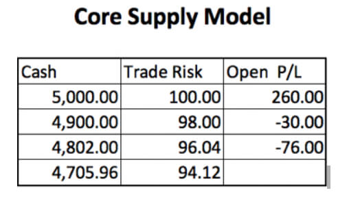
Using this guideline, you determine the dollar risk for the next trade by taking the remaining cash left on your account. For example, your initial account cash balance is $5,000, and you have risked 2% (or $100) in your first trade. To compute the next position size, you should consider the $4,900 remaining cash; thus, if your position sizing method told you to use a 2% risk, the size of your next trade should be $4900 *2% or $98.

Using the Core Supply Model, open profits are not considered until the trade or trades are closed. The formula subtracts all the initial risk of the previous trades until the trades are closed. New positions are always computed using the cash calculated with the formula:

Cash = Total equity – Open-trade risks

Balanced Total Supply Model

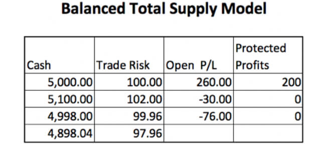
This method is similar to the Core Supply Model, but it adds the profits of the positions in your favor, but only if a stop-loss level protects them. For example, let’s assume you currently have a paper gain of $260 in your first trade, as in the following figure, and you’ve placed a trailing stop that is now protecting $200 of it. In this case, the available cash for the second trade will be $4,900+$200 = $5,100.

Total Supply Model

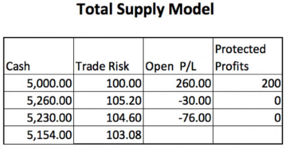
The total available cash is calculated by adding and subtracting all the open positions’ gains and losses. This model is a bit riskier than the previous model, as all the profits are added without the requirement of protecting them with a stop-loss. This makes it very simple, although it delivers slightly larger sizes. If we use the previous table, the $250 current profit on the first trade will be entirely added to the $4,900 base supply for a total supply of $5,150 available for the next trade.

This risk model is very much used by account managers, as it helps them keep their position size (their risk) constant, because the next trade size it will always be a percentage of the total available equity.

Boosted Supply Model

This model is made of two “pockets”: The Conservative Money Pocket and the Boosted Money Pocket. This central approach uses a low-risk sizing model on the Conservative Money Pocket and an expanded risk sizing model on the Boosted Money Pocket. The Boosted Money Pocket can be filled using two methods. The first one is to allocate a percentage of the equity ( from 5% to 20%) to the Boosted Money Pocket. The second method is to wait for “market money.” Market money is money resulting from your net gains.
The Boosted Supply Model’s main idea is to be conservative with most of your trading funds and be speculative with the market’s money or a small part of your equity.
Also, the key to this methodology is that the Boosted Money Pocket be rebalanced. We can set a rule to rebalance every week, 15 days or one month, or set a profit target for this pocket that, when reached, will trigger a rebalance action to set it to a pre-defined 5%-20% level.

Using this boosted model, a trader is willing to set a max drawdown much higher to profit from the accelerated equity growth. It is well known that equity growth grows in a geometric progression while drawdowns move in an arithmetic progression. That means that we could obtain over 10X equity growth with just a 2X drawdown increase. We will develop more on this with specific models in future videos. But, as an example, if a trading system delivers a 10% drawdown using 1% position sizing, a boosted pocket could be set to 6X this risk (6%) for a 60% projected drawdown on this 10% portion of the funds of the market’s money. That would triple the profitability of the system but remaining conservative on the core funds of the trader.

Categories
Forex Videos

Forex Position Sizing – The Gamblers Fallacy!


Position Size II- The Gamblers Fallacy

We are going to commit this video to explain a gross misconception about streaks. The majority of traders tend to think that the chance of the next trade being a winner or a loser depends on the previous events. That means people feel that long streaks have a high probability of ending in the next trade. That belief is wrong and makes many traders think that adapting his position size to the recent performance is the right way to go.


Dependent or independent probability events?
What is a dependent probability event?
A dependent probability event is an event whose probability of outcome depends on the previous results. For example, the likelihood of getting an ace on a deck of cards depends on the previous draws. The initial probability is 4/52, but as the game evolves and more cards are drawn, it will depend on the number of cards left and the number of ace cards drawn. So, if the deck currently has 41 cards and one of the aces had been drawn, the odds of the next draw being an ace is 3/41.


Independent probability events

An independent probability event is an event whose probability of outcome does not depend on the previous results. Coin tosses and dice rolling are among this kind of events. The odds of a fair coin resulting in heads (or tails) is not dependent on the previous results, even when many people believe that a streak of heads has a higher chance of ending with the next move than when the last play was a tail. In fact, the odds of a streak to end are the same in all situations, no matter how long the streak is: 50%.

Trading is a game of chances.


The question is now to decide is if a trading strategy is a dependent or an independent process. That is a very interesting question, and it is difficult to answer with 100% accuracy. The majority of the strategies are independent processes, meaning the next trade outcome is not dependent on the preceding trades. That means it has no memory. Also, to prove a trading system is dependent is very hard to accomplish, and it is left to errors.

Modulating the position size

It would be nice to trade a dependent system. Imagine you know the odds of a win are higher when the previous trade was also a win. You could increase your position after a win, and decrease it after a loss. On a system in which the odds of winning after a win drops, you could do the opposite: reduce your position size after a win and increase it after a loss.
But modulating the position size can be wrong if the trading strategy or system shows independency, and that is what is called the gambler’s fallacy: People tend to believe the odds of the next move change with past events when, in fact, it did not. That makes them adapt their position in the wrong way. They tend to reduce their position size during large winning streaks and increase it during losing streaks, expecting a winner soon. That is the opposite of cutting losses short.

Streaks cause doubt on traders

The majority of traders follow their strategy with little confidence. Since they don’t fully understand the statistical principles behind streaks, they abandon the system after four or five consecutive losses, thinking that the markets have changed or that the system’s testing was not as good as they thought.

Changing the risk

Another dangerous situation may occur on a winning streak, in which the trader may think that his system is infallible, thus increasing the size and risk of the next trades. In his Definitive Guide to Position Sizing, Van K. Tharp explains a curious situation that happened when they were testing their “Position Sizing Game.” The game was set to 60% winners where 55% of the time, they won what they risked, and 5% of the time, they won 10 times their bet. One of their testers had an incredible 23 winning streak, after winning ten times in a row, the tester began to increase the trade size from 10% to 95% bringing $10,000 to 1.45 million in 23 trades. On trade #24, the tester risked $1,000,000 and lost, leaving the trading account balance with just $45,000.

The lesson is evident. Events subject to the laws of chance have winning and losing streaks that defy the common understanding of people.
We should leave a more in-depth analysis of streaks for another video, but suffice to say that the odds of a streak is conditioned by the probability of a single event.

The odds are out there

The ods of an n streak are P ^n that means, P multiplied by itself n times, where P is the probability of the event. For instance, the odds of a four heads streak on a fair coin toss are 0.5×0.5×0.5×0.5 = 0.0625 = 6.25% .
That means the larger the probability of a single event happening, the higher the odds of a large streak.

Translated to the trading world, a system with a high percentage of winners will have short losing streaks and extended winning streaks. The opposite is true. A trading system with a low percentage of winners will suffer larger losing streaks.

Categories
Forex Market Forex Risk Management

These Are Some Of The Best Position Sizing Techniques You Should Know!

Introduction

In our previous article, we addressed the concept of position sizing, drawdown, and techniques. Now we extend this discussion and look at other crucial aspects of position sizing, which are very important. In this article, let’s determine how one can position themselves in the forex market based on three different models. Each of these has its own merits that impose some sort of position sizing discipline in traders.

The three core position sizing techniques in terms of risk are:

  • Fixed lot per amount
  • Percentage margin
  • Degree of volatility

These models can be applied to all the asset classes and are time frame independent.

We suggest you stick to one model to estimate the position size or at most two position sizing techniques. Following every given method will increase complexity, and that is not good for a trader.

Fixed Lot Per Amount

This is a fairly simple model. It requires a trader to simply state how many lots he is willing to trade for a given amount of capital. For example, let us assume a trader is having $2000 in his trading account, and he trades only the major currency pairs like  EUR/USD, GBP/USD, GBP/JPY, USD/JPY, etc.

The trader simply needs to make a thumb rule that he/she will not trade more than one standard lot of futures (of major currency pairs) per $2000 at any given point.

The lot size can also be determined based on their risk appetite and money management principles. This technique of ‘fixed risk’ is based more on the discipline than strategy.

Percentage Margin

This position sizing technique is more structured than the ‘Fixed lot per amount’ technique, especially for intraday traders. It requires a trader to position themself based on the margin. Here, a trader essentially fixes an ‘X’ percentage of their capital as margin amount to any particular trade. Let’s see how this works with the help of an example.

Assume a trader named Tim has a trading capital of $5000; with this, he decides not to expose more than 20% as margin amount on a particular trade. This translates to a capital of $1000 per trade.

Now, if Tim gets an opportunity in another currency pair, he would be forced to let go of this margin as it would double to 40% (20% + 20%). This new opportunity will be out of his trading universe until and unless he increases his trading capital. Hence, one should not randomly increase the margin to accommodate opportunities.

The percentage margin ensures a trader pays roughly the same margin to all positions irrespective of the forex pair and volatility. Otherwise, they would end up in risky bets and therefore altering the entire risk profile of their account.

Degree Of Volatility

The degree of volatility accounts for the volatility of the underlying asset. To measure volatility, we make use of the ATR indicator, as suggested by Van Tharp. This position sizing technique defines the maximum amount of volatility exposure one can assume for the given trading capital.

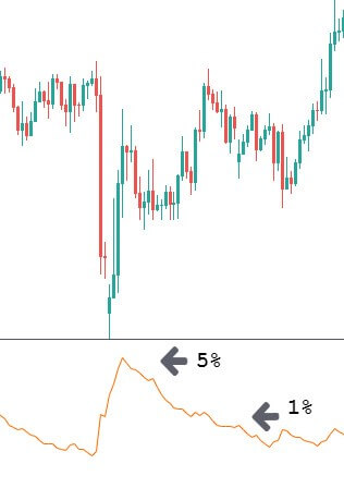
Below we have plotted the ATR indicator on to the USD/JPY forex chart.

The 14-day ATR has a peak and then a decline, which shows a decrease in volatility. As you know that high volatility conditions are the best times to trade (less slippage, high liquidity, etc.), you can risk up to 5% of your trading capital on the trade while one should not risk more than 1% when the ATR is at the lowest point. Do not forget the risks involved while trading highly volatile markets. Only use this position sizing technique when you completely trust your trading strategy.

Conclusion

A trader should not risk too much on any trade, especially if their trading capital is small. Remember, your odds of making a profit are high when you manage your position size and risk the right amount on each of the trade you take.

Beginners should trade thin to get experience with open positions, so they can assess the stress of a loss and gradually increase the position size as he is comfortable with the strategy results and performance. As a matter of fact, this is also the right way to proceed when trading live a new strategy, be it a beginner or an experienced trader.

Cheers!

Categories
Forex Market

Understanding Drawdown & Its Relation With Position Size

Introduction

Do you know that there is a safe way to choose the maximum lot size when you trade? That too while keeping your account safe from blowing when a losing streak of trades occur? To constantly stay in the game and be able to recover from losses requires patience, clarity, and, more importantly – optimal Position sizing. The position size in simple words is how much a trader invests in each trade. There are different models deployed to reach the optimal position sizing depending on the objective of the trade. Before that, let’s first understand what drawdown is and how it is related to position sizing.

What is the maximum drawdown?

The maximum drawdown is the biggest drop in the accumulated profit chart and, consequently, that of the trading capital. Imagine a situation where a trader had 200 pips in profit after a number of trades, and on the following days’ profit dropped to 136 pips before he can make new accumulated high.

So, the drawdown here was 200-136 = 64 pips

When this drawdown increases, it reaches a level (negative drawdown), after which it becomes impossible to trade (due to loss of trading capital). Maximum drawdown is the loss that the trader can take in order to survive in the market and be able to continue trading.

How is drawdown related to position sizing?

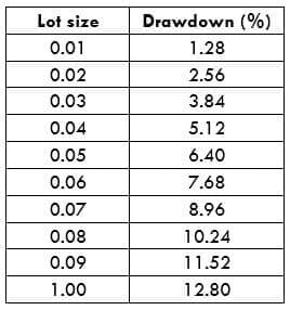
Taking the above example, let us assume that the trading capital was $500 and the trader trades with a lot size of 0.01. The drawdown he experienced was 64 pips, which is $6.4 (1 Pip = $0.1). So the amount of money he/she risking in this trade is 6.4/500 x 100 = 1.28% of the account size.

Now let us see how this drawdown increases with a change in position size.

How much drawdown can I handle so that it doesn’t affect the mental state and my trading style?

As you can see below, the drawdown % increase as the lot size increases and the account gets into an unsustainable state (Especially when the Trading Capital is $500). Hence you need to calculate risk based on your risk tolerance drawdown.

The right way to look at drawdown and position size

Typically, the drawdown occurs after a series of consecutive losses. The very first thing a trader needs to do is to analyze and figure out the number of losing trader he/she can endure. Depending on that, the maximum risk percentage should be defined. So essentially, this percentage is the maximum amount of trading capital a trader affords to lose. If the losses cross this percentage, his/her account get unsustainable.

For instance, I can bear a maximum drawdown of 20%. So I should be willing to design a strategy and chose my trading size in such a way that it is very unlikely for me to reach the 20% drawdown. Let’s denote the number of losing streaks as N. I should make sure that my strategy has a winning percentage of at least 50% or more with high RRRs. Let’s assume the maximum number of losing streaks I can afford is 10 (i.e. N=10).

Dividing the maximum drawdown (20%) with N (10) gives 2%. This means that I cannot risk more than 2% of my trading capital on a trade to sustain in the market. If I have more than one open trading position, I should be distributing the risk among all of the open positions. So here, if I have 2 open positions, I shouldn’t be risking more than 1% in each of the trades. This is one of the best ways to look at drawdown and position size.

Different approaches to position sizing

Defined Percentage Risk

In this position sizing strategy, we risk a fixed percentage of the trading capital (e.g., 1%) for each trade. This is followed by most of the traders across the world and it is pretty simple to use as well. Essentially, the trader is required to put the stop-loss more accurately and not randomly to prevent the stop-loss hunt. This might sound pretty easy but it needs a lot of discipline to overcome the greed and not raise the position size when you see a clear profitable trading signal.

The Kelly Criterion Model

John Kelly described this criterion pretty long ago, which computes the optimal position size for a series of trades.

Kelly Percentage = W – [(1-W) / R)

Where, W – Winning probability and R – Profit/Loss ratio

When a trader keeps a record of all their trades, they can calculate their winning probability and profit/loss ratio. Then, they can use them in the above equation to calculate the optimal position size.

Conclusion

You now know the importance of position size and its relation to drawdown. By using this, leverage can also be used appropriately to avoid blowing-up your account because of the drawdown. By doing this, you can maximize your earnings and reduce drawdown to an acceptable value.

Our suggestion for you is to use a trading strategy for a long time. If a strategy hasn’t been tried many times, the big drawdown might not have appeared yet. The bigger the history of using the strategy, the more confidence you will get to increase the lot size. Cheers!

Categories
Forex Risk Management

Basics of Risk To Reward Ratio In Forex Trading

Introduction

The Risk to Reward Ratio is one of the most critical aspects of risk management in Forex trading. Traders with a clear understanding of what RRR is can improve his/her chances of making more profits. In this article, let’s discuss the fundamentals of Risk to Reward ratio with examples and also the ways through which it can be increased while taking your trades.

What is the Risk to Reward Ratio?

Before getting right into the topic, let’s define the meaning of ‘Risk’ here. Risk is the amount of money that a trader is willing to lose in a trade. If you have read our previous money management articles, we mentioned that a trader should not be risking more than 2-3% of their trading capital in each trade. It means when they find a trade setup, they should choose their position size in such a way that if the market hits their stop-loss, they lose a maximum of 2-3% of their trading capital.

Now, the Risk to Reward Ratio is simply the ratio between the size of your stop-loss to the size of your target profit. Let’s say your stop-loss is five pips away from your entry price and your target profit is ten pips away from the entry. In this case, your risk to reward ratio is 1:2 (5 Pips/ 10 Pips).

The larger the profit against the stop loss, the smaller the risk to reward ratio. Which means your risk is a lot smaller than your reward.

What is the recommended risk to reward ratio in the forex market?

Typically, a minimum of 1:1 or 1:2 RRR is recommended for novice traders. There are super conservative traders where they look for a minimum RRR of 1:5.

The risk to reward in every trade cannot be fixed as it varies depending on the market condition. For example, 1:3 or 1:5 RR ratio is achievable when the market is trending, and you enter the market at the right time. Whereas when the market is not very volatile, we should be happy with a risk to reward ratio of 1:1.

How to increase the risk to reward (RR) ratio?

🏳️ Raising target and putting stop-loss to breakeven

A trader can think of raising the target if the market moves to the initial take-profit quickly. This is because when the market moves so fast, it has the potential to move further, thereby increasing the profits.

🏳️ Finding trade setups from the larger time frame

Another way to increase the risk to reward (RR) ratio is by taking the strong trade setups from the higher time frames like daily, weekly, and monthly. We need to wait for such strong trade setups to form. Once formed, the price will move for hundreds of pips, and so we can have wide targets.

Final words

Higher the RRR, the better it is, and of course, higher RRRs are more challenging to achieve. So, do not forget to keep the expectations real and the risks appropriate. You do not have to avoid perfect trades just because the RRR is not as high as 1:5. Make sure to do proper risk management before placing a trade. Never trade with a risk to reward ratio that is too less and try to maximize it as much as possible. Cheers!

Categories
Forex Videos

Why You Will Never Be A Successful Forex Trader – Understanding Forex Position Sizing

Position Sizing

Position sizing is the technical size of a trade, or the monetary risk, that a trader is going to take in any given trade. Investors use position sizing to help determine how many units of a particular currency they can purchase, or sell, which helps to control risk and help maximize returns.
Let’s face it, some people might be prepared to go into a casino and put all of their available funds on black, or red, or odds or evens, or a select a number on the roulette wheel, or snake eyes on a throw of the dice, and then hope for the best! A few lucky punters might win occasionally. However, the house always wins in the end!

In Forex trading, we are unlike a casino, insofar as we use fundamental and technical analysis skills in order to try and stack the odds in our favor. We then utilize position sizing in order to maximize our winning potential and also to help to mitigate against the risk of losing trades. In other words, if we do suffer a few losses, we live to fight another day, unlike gamblers who put all their money on one roll of the dice.
Therefore, traders must put up an appropriate amount per trade, given their level of experience, the level of volatility in the market, and proportional to their account balance size. This is where most inexperienced traders go wrong; they simply use too much of their capital per trade, and as a result, when they have a couple of losing trades, they blow their accounts. Statistically speaking, over 70% of new retail forex traders will blow their accounts within the first six months. This, coupled with a lack of understanding of how the forex market works and a lack of understanding regarding leverage and margin requirements, is the account killer for new traders.

In order to be a successful Forex trader, they must learn how to apply the correct use of capital exposure per trade or position sizing. The three most important issues are 1: how much capital they wish to assign to each trade, 2: what is the trade risk associated with each trade, and 3: are they calculating position size accurately.
All of these issues come under effective risk management and are just as important as any other area in Forex trading, such as technical and fundamental analysis. If traders do not understand this, then everything else they know about the market is a waste of time! In Forex trading, every aspect must work together in unison, in order for a trader to consistently win trades. When it comes to trading, capital preservation is paramount to survival.

Example A


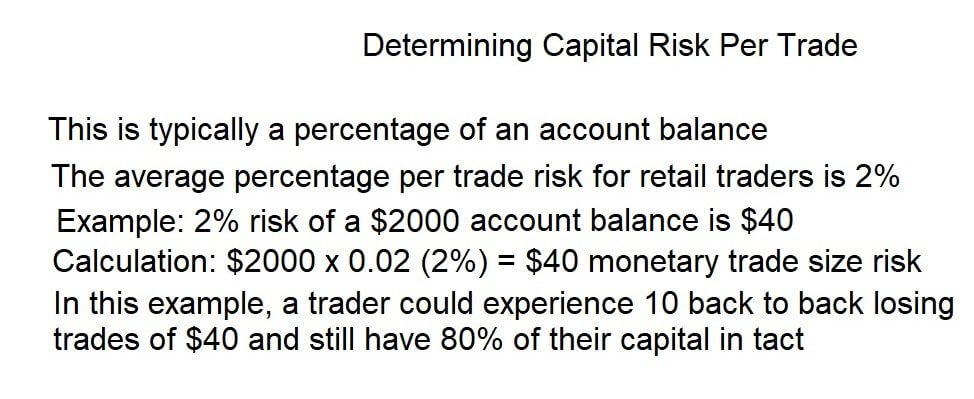
Let’s look at example A: Determining capital risk per trade This is typically a percentage of an account balance
The average percentage per trade risk for retail traders is 2%
Example: 2% risk of a $2,000 account balance is $40
Calculation: $2000 x 0.02 or 2% = monetary trade size risk
In this example, a trader could experience ten back-to-back losing trades or $40 and still have
80% of the capital intact.

It is extremely advisable that new traders adopt this very important position sizing risk strategy, in order to achieve longevity in their trading careers, especially in the early stages. Once a trader has a consistent winning methodology in place percentage risk per trade can be gradually increased above 2%. Traders are also advised to try and achieve a minimum of 2 to 1 win to loss ratio. This would mean that a trader should be looking to make a minimum of $80 per trade win while risking a $40 loss.

Example B

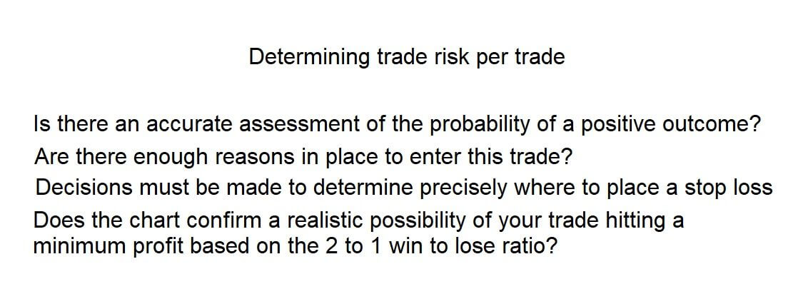
Let’s look at example B: Determining trade risk per trade
Is there an accurate assessment of the probability of a positive outcome?
Are there enough reasons in place to enter this trade?
Decisions must be made to determine precisely where to place a stop loss
Does the chart confirm a realistic possibility of your trade hitting a minimum profit based on the 2 to 1 win to loss ratio?
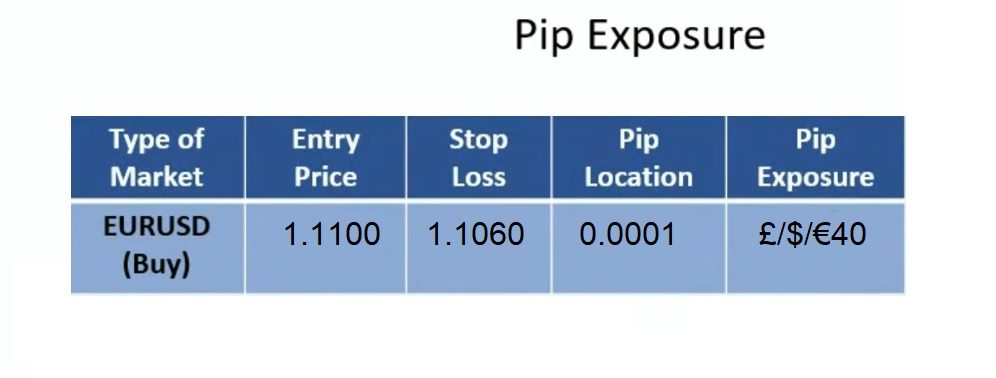
One area where new traders fall down is their failure to understand that when they trade in the Forex market, they trade on a per pip basis within exchange rate fluctuations. That is to say, that traders’ winnings and losses are calculated on the movements of pips. In Forex, trading pips are calculated from four places to the right of the decimal point.

Example C

Therefore in example C, if we bought 1 mini lot of the EURUSD pair at 1:1100, we would need to place our stop loss at 1.1060, which would give us an exposure of $40.
In keeping with our 2 to 1 win-loss ratio, we would put our take profit at 1.1180.

Example D

Let’s look at example D: Notional trade size.
In order to understand position sizing, traders also need to understand the notional size of a trade. In keeping with our earlier EURUSD trade example, when setting our trade size on our platform, we need to understand about lot sizes. Therefore when trading currencies, because we are trading on leverage, essentially when we trade one mini lot, we are effectively trading 10,000 units of the base currency of the particular pair.
And so in our example, we would be buying 10,000 units of Euros, as the base currency is always quoted first, and the counter currency is always quoted second.

Categories
Forex Daily Topic Forex Money Management

Things you should Know about Leverage, Drawdown and Risk

Novice traders usually prefer to focus on trade ideas and strategies, believing that the path to success is the knowledge about entries and exits. But in a trading environment with leverage, risk management plays a crucial role. This article tries to show why.

Key points

 In trading, There are two key points a trader must care and make sure:

  1.  That his strategy is good
  2. Risk management trough proper position sizing

Good Strategies and Bad strategies

The first thing to consider is the quality of the trading system or strategy. There are risk management ideas that might convert a losing system into a winner if the problem was that stop-loss settings were wrong, But no position sizing can change a losing strategy into a winning one. Therefore, the first thing a trader should care about is for his system to have a positive edge.

In statistical terms, the strategy should have a positive expectation. If not, the trader should analyze it, find the weak points, and modify it for profitability. Once the system is profitable, it can be traded. Finally, depending on its quality, the system will make grow the trading account fast or slow, and, also, its growth can be optimized through position sizing.

Strategy basic Statistical 

To analyze a trading strategy, we need to normalize its trades to a basic unit and, then extract its four main statistical parameters:

  • Percent winners
  • Mean reward-to-risk Ratio
  • Mathematical expectation
  • Standard Deviation of the expectation.

For example, the system we are going to use as an example in this article shows the following parameters:

STRATEGY STATISTICAL PARAMETERS : 

  •  Nr. of Trades: 143.00
  •  Percent winners: 58.74%
  •  Mean Reward Ratio: 1.22
  •  Mathematical Expectation: 0.0887
  •  Standard dev: 0.4090

It is not a really good system, but it’s tradeable. The Mathematical expectation says that the system, using a basic unit of risk of one dollar, is able to extract a mean of 8.87 cents per dollar risked on every trade. Therefore, the system has an 8.87 cents edge against the market, which is 8.87%.

Drawdown

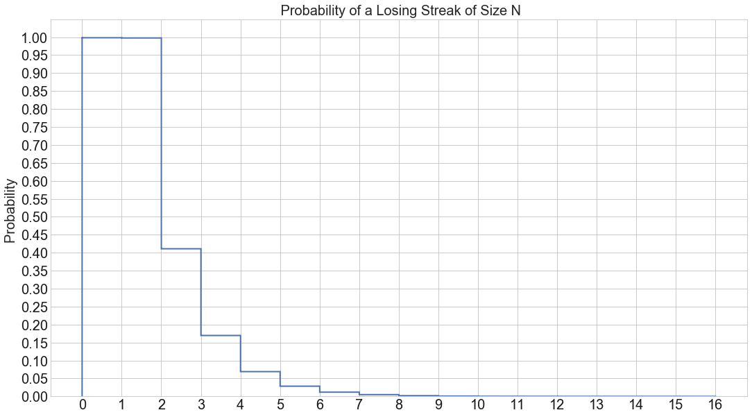
You can see that here, we did not show the drawdown as a parameter to consider. That is because drawdown is dependent on position sizing. The parameter we can compute, though, is the losing streak, which is the number of continuous losses we could expect based on the percent of losses. As we know, the percent of losers is 1-percent winners. Therefore, in this case, Percent losers = 41.26%

With that information, we can create a probabilistic curve of a losing streak of size N, such as the one here. But the trade size is what is going to define the drawdown parameter.

Fig 1 – Losing Streak Probability Curve

Leverage and Drawdown

Forex is a leveraged trading environment, and many brokers offer its customers the ability to go up to 500:1, meaning traders can use up to 500x the size of its trading account to open positions. But is it wise to get that leveraged? Let’s do an experiment using the above-mentioned system.

As said above, the system has been taken from a real trader and is a good, although not brilliant system. But it is a real no-hype system that can be traded what we want to test. For this test, we will always start with a balance of $10,000 and will increase the trade size using the same trade segment. 

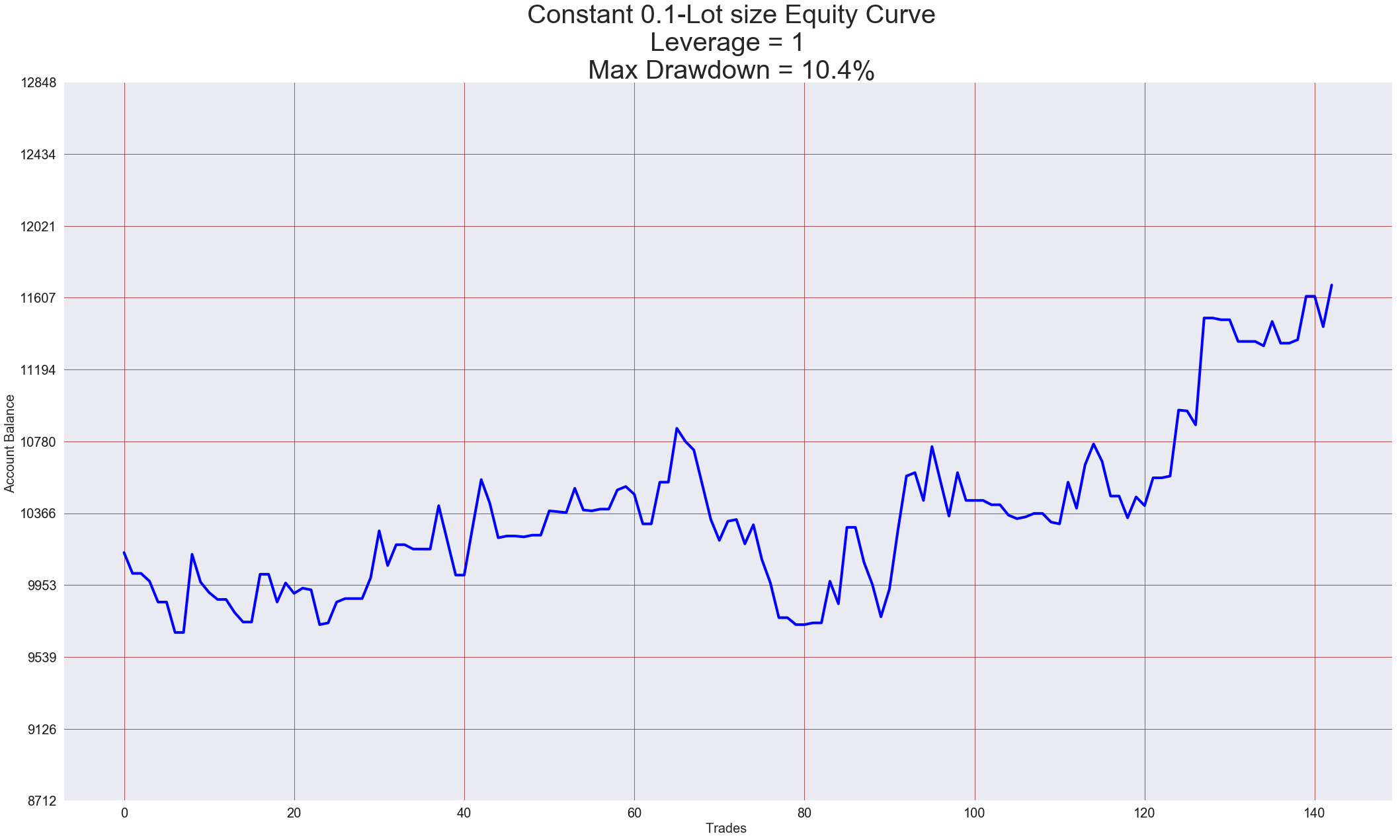
Leverage = 1

Fig 2 – 0.1 Lots per trade

Using a leverage of one, we see that the system shows a max drawdown of 10.4 percent, and the final equity after 143 trades is a bit more than $11.600, which is 16% growth.

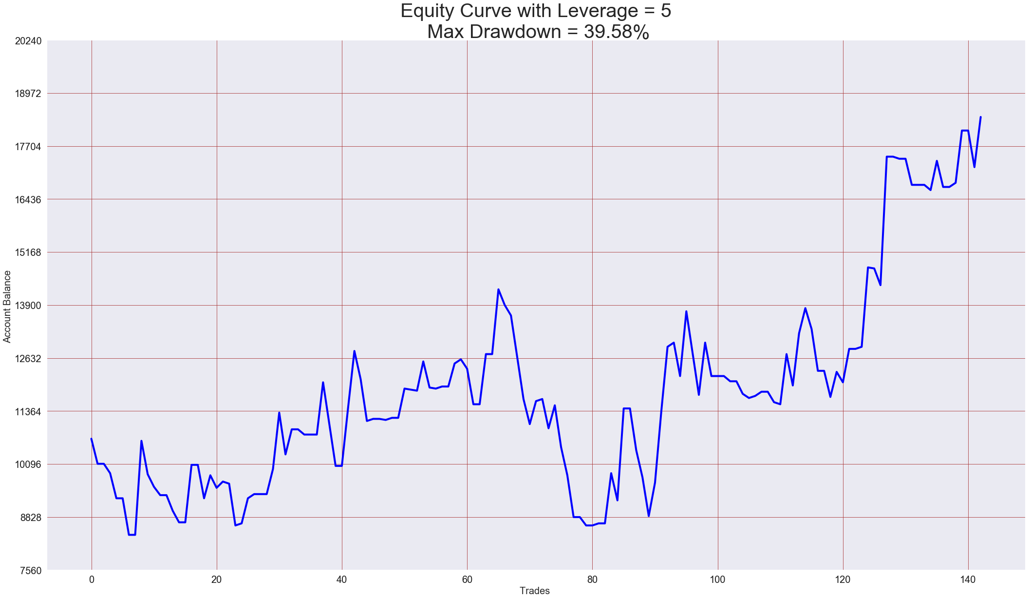
Leverage = 5

Fig 3 – 5X Leverage

Using 5X leverage, we notice that the Max Drawdown went to 39.58%, and the final equity ended up at $18,400.00 for an 84% profit.

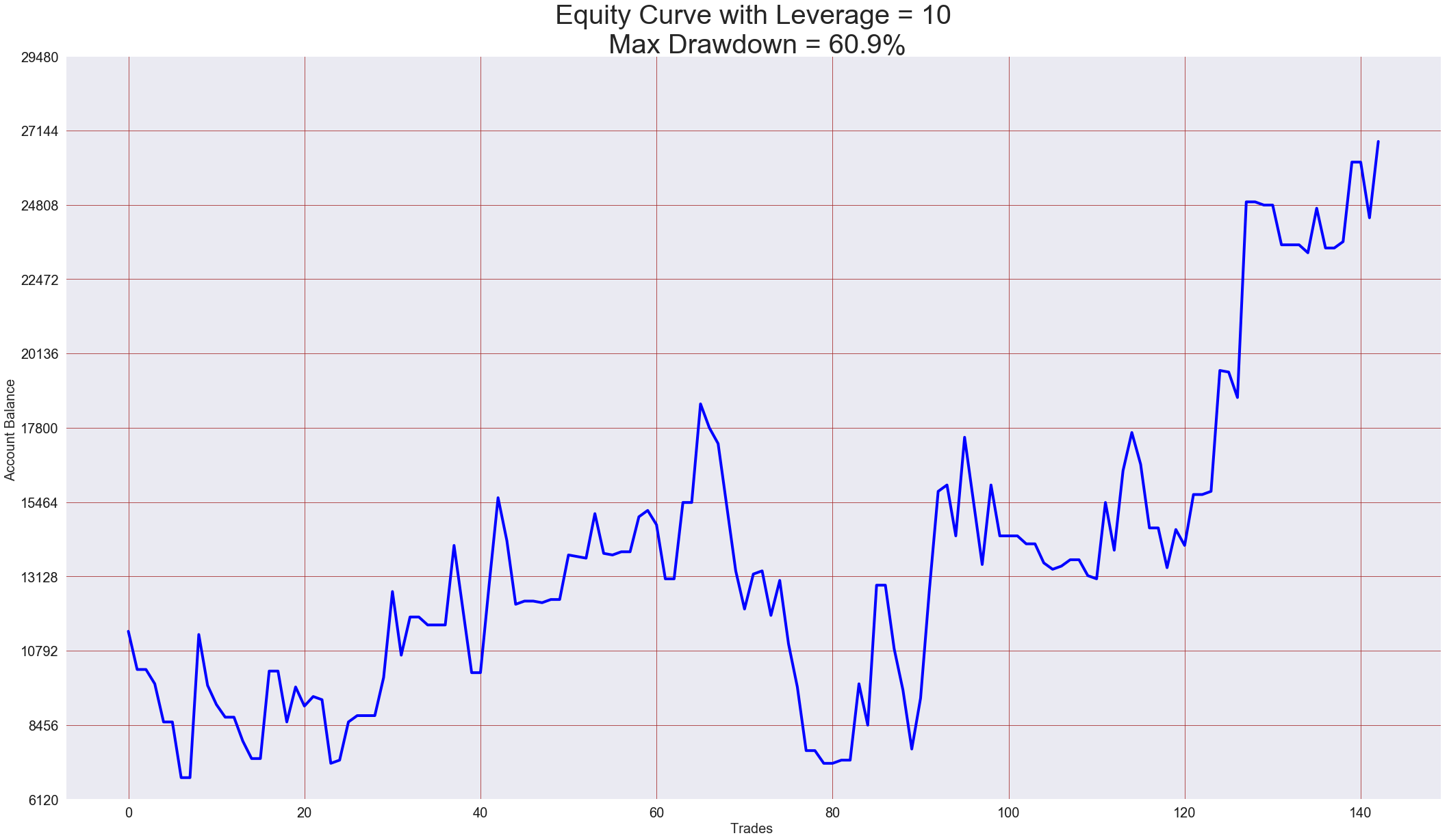
Leverage = 10

Fig 4 – 10X Leverage

If the trader dares to go to 10X leverage, he must endure close to 61% drawdown for the opportunity to receive 168% profit and a total equity of $26,800 at the end of a 143-trade cycle.

Leverage = 20

Fig 5 – 20X Leverage

Leverage 20X is even wilder. The trader has to withstand up to 83.4% drawdown for a gain of 336.00 % profit.  The question is when to stop? Will a 40X leverage be even better for the profit-hungry trader?

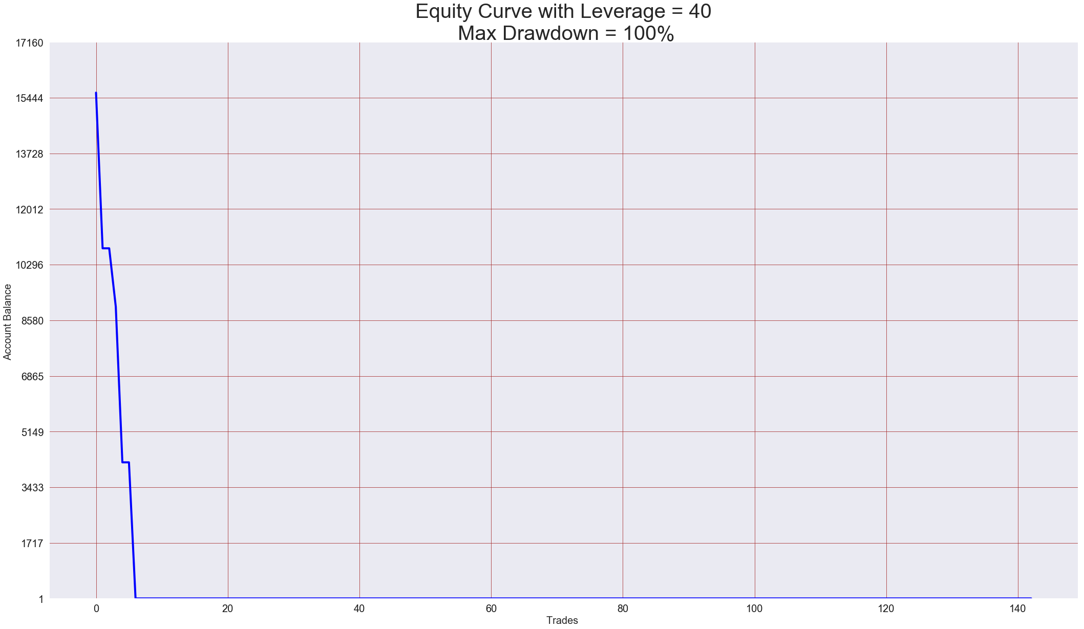
Leverage = 40

Fig 6 – 40X Leverage

We can see that at some point, the risk is too much, and a profitable system, with the wrong risk and size management, can be converted into a very fast losing system and wipe the entire account.

As we see here, a 40X leverage is wild enough to wipe an entire account using a very profitable trading system. We must understand that up to one point, increasing the leverage will increase risk while decrease profitability.

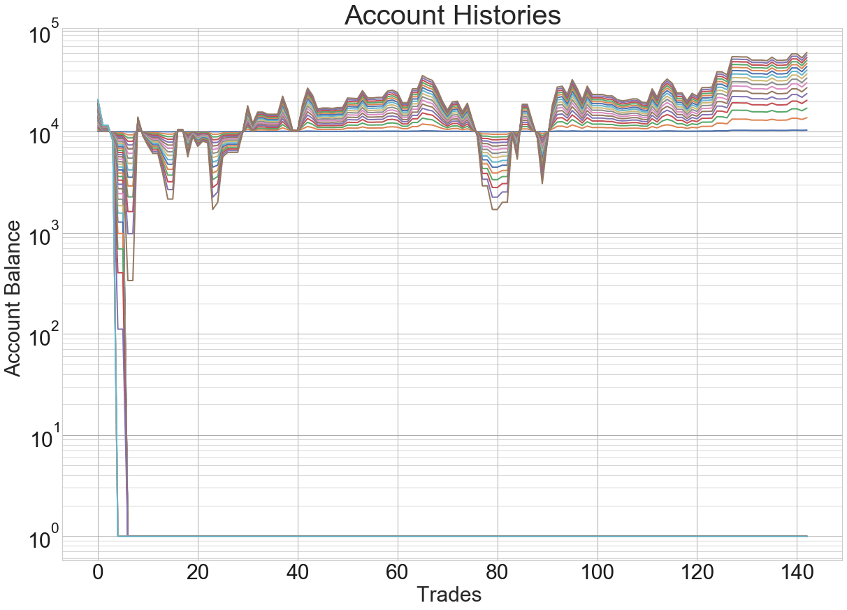
As a summary, let’s see the plot of several account histories with increasing leverage

Fig 7 – 40X Leverage

This time we have plotted the histories on a semi-log scale to be aware of the enormous scale of the drawdowns. On the graph, we can see that the most critical moment of the histories happens at about trade Nr. five or six, which crashes all accounts above 30X leverage. But, if we take this event aside, we can see that to reach its destination traders must endure four more events when they lose close to 80% of their initial funds. We must take into account that at the moment of these events happening, there is no way to know when will they stop and start recovering the funds back.

A Propper Attitude Towards Risk

Position sizing and risk management are the tools traders have to accomplish their trading objectives, but it has to be done correctly.

We first need to set the daily, weekly, or monthly profitability of the trading strategy. Let keep using the previous example.  We know that the system has a mean of 8.87 cents per dollar risked.  Let’s suppose the system has an average of six daily trades. Then, the profitability of this system is $0.53 daily, and $10.64 monthly per dollar risked.

From the losing streak curve, we see that it is wise to be prepared for a max streak of, at least eight losing trades.  Then, we define our comfort zone for drawdowns. Let say we are bold and wanted to risk up to 40% of the capital. To accomplish this, we divide the max 40% drawdown by our defined max losing streak of 8, and the result will be the maximum percent risked on every trade. In this case, Risk per trade = 5%. (That is a huge of risk, we do not recommend more than 1%, by the way).

Now, if your current account balance were $10,000,  the risk per position should be 5% * 10,000, = $500. With that information, we can see that the system would deliver $5,320 monthly, on average.

If we were to double this amount, we would need to double the account balance or wait roughly two months until the profits reached the $10K mark.

The concept of applying a trade size proportional to the account balance helps traders to apply compounding growth to their accounts, while automatically reducing the trade size while in a losing streak on a dollar basis. More on compound growth will be developed in a future article.


Categories
Forex Market

What Is Pip & Why Should You Know About It?

What is a pip?

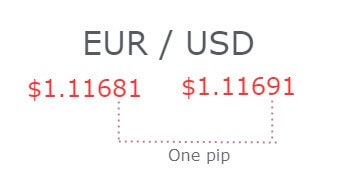
Essentially, a pip represents the price interest point. It is known to be the smallest numerical price move in the forex market. As you know that most currencies are priced to 4 decimal places, obviously, any change in price would start from the last decimal point. For example, in the price quote, $1.0002, ‘2’ indicates the pip value. A pipette means the 5th decimal place, while pip is the 4th decimal place.

For most pairs (except JPY), it is equivalent to 0.01% or 1/100th of one percent. In the forex market, this is referred to as Basis Point (BPS). One BPS is equal to 0.01% and denotes the percentage change in the exchange rate.

Calculation of move

Now that you know what pip means, let us see how it changes the profit and loss in your trading account. Large positions will have greater monetary consequences in your balance. The formula for calculating the value of the position is:

Position size x 0.0001 = Monetary value of pip

Let us use the above formula and apply it in some real pairs. If you open a position of 1000 units, the pip value can be calculated as 1000 (units) x 0.0001 (one pip) = $0.1 per pip.

When you open buy positions and market reacts in your favor, for every pip movement, you will earn $0.1, and the same is the case for a sell position. If the market moves against you after you buy or sell, $0.1 will be lost per pip movement as the trend continues in the opposite direction. Increasing or decreasing the number of positions will have the exact effect on the pip value.

Different currencies and their pip value

Pip value varies per currency as they are dependent on how it is traded. It also depends on the trading platform and the price feed. It is important to know that there are brokers who show four digits as pip, and some show five. One of the most important points you need to know is the average daily trading range, in order to gauge volatility in the market.

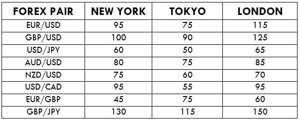
Average daily pip movement of major currency pairs

Conclusion

To conclude, pips are the smallest increment by which a currency pair can change in value and represents the fourth decimal of a currency pair other than the Japanese yen. In the case of Japanese yen, the pip is located at the second decimal place. Proper knowledge of pips will help you determine your stop loss size, as it is a major part of any strategy. One should never underestimate the simplicity of pip. Now that you have learned what a pip means, you can proceed to more trading concepts. Cheers!

Categories
Forex Educational Library

The Power Of Compounding


Novice traders enter the Forex markets with the illusion of becoming independent and wealthy. And they may be right. So why 95% of forex traders fail?

After no trading plan and psychological weaknesses and biases comes Too high position sizing as the main cause for failure.

I guess that the become rich quick mentality, an evident psychological weakness, drives them to trade big at the wrong time. Then Fear and greed make the rest.

Therefore, my first recommendation for a new trader is to doubt about his strength to support the psychological pressure to break his system. That is much better accomplished if he or she risks small amounts. The initial two years of trading should be dedicated to learn and practice the needed discipline to respect the trading rules.

The power of compounding

To help you take out your anxiety for a quick buck profit, Let’s analyse the power of compounding.

Let’s first see, graphically an account of 10,000 € grow at a monthly rate of 0,083%, a nominal annual rate of 1% for 50 years (600 months):

Well, we observe that this state of affairs is only good for the bankers. It takes 50 years to grow 10K into 16,500K. That’s the reason we are willing to risk trading.

Let suppose we get  a risk-free 10% annual return instead, again, with monthly payments of 10%/12:

That is becoming interesting. One, we need to wait patiently for 50 years to become millionaires, and, two, we don’t know how much of that will be erased by inflation.

Let’s suppose we are investing ala Warren Buffett with an annual mean return of 26%, that, also steadily grows on a monthly basis. In this case, the graph is presented in semi-log scale for obvious reasons. The x-scale is in months while the y-scale says how many zeros has the account balance. For instance, 106 means the account has 1 followed by six zeros:

Now, that is another history! We see that in 50 years we will be as filthily rich as Warren Buffett et al. !  We observe, also, that we add one zero to our account roughly once every 100 months. Not Bad. We multiply by ten our stake every two years! And that is achieved with a mean monthly rate of return on our capital of 2.17%, which means we just need to make sure we get a daily return of 0.11%.

The problem is within us:

This one is the same equity curve than the previous one but in a linear scale. We observe that it shows an exponential line, and there resides our psychological problem: The net equity grows relatively slow at the beginning. We need four years to reach six zeros, but in another four years, we will be close to eight. That shows that the power of compounding is a long-distance race, not a sprint.

The other side of growth

Things are not that perfect in trading. We don’t see nice curves up to richness. We should expect not only run-ups but, also drawdowns. Let’s observe the equity curve of a typical system using a nominal risk of 0.5% which takes, for simplicity, one trade per day, or 20 per month. And let’s put a magnifying glass on the first year of its history.


   Starting Capital:  10,000
Mean ending Capital:  11,817
     Capital % gain:  18.17%
       Max drawdown:  2.64%

This is a real system, achievable, with the basic statistics as follows:
STRATEGY STATISTICS:
              Nr. of Trades: 143.00
                    gainers: 58.74%
              Profit Factor: 1.74
                   mean nxR: 1.22
 Sample Stats Parameters:
           mean(Expectancy): 0.3070
               Standard dev: 1.9994
            VAN K THARP SQN: 1.5353

The monthly mean profit, using a 0.5% risk is 1.5%, which gives an annual growth of 18%. A bit less than what Warren Buffet has been performing. The nice feature is that using a 0.5% risk the max drawdown is 2.64%. Now, let’s see how fare this system, using exactly the same trade percent results when risk rises  because we increase the position size:

2% Risk:

   Starting Capital:  10,000  
Mean ending Capital:  18,910      
     Capital % gain:  89.10%      
       Max drawdown:  10.38%


5% risk:

     Starting Capital:  10,000
  Mean ending Capital:  42,615
       Capital % gain:  326.15%
         Max drawdown:  25.39%


10% Risk:

     Starting Capital:  10,000
  Mean ending Capital:  118,032
       Capital % gain:  1,080.32%
         Max drawdown:  47.67%


20% Risk:


     Starting Capital:  10,000
  Mean ending Capital:  308,888
       Capital % gain:  2,988.88%
         Max drawdown:  79.99%

35% Risk:

   Starting Capital:  10,000
Mean ending Capital:  124,613
     Capital % gain:  1,146.13%
       Max drawdown:  96.83%

45% Risk:


   Starting Capital:  10,000
Mean ending Capital:  14,725
     Capital % gain:  47.25%
       Max drawdown:  99.53%

 Conclusions:

From the above examples we take that:

  1. Max drawdown is related to position size. The bigger its size, the higher the drawdown.
  2. As position size grows, up to a certain limit, capital gain grows geometrically, but drawdowns grow also, although arithmetically.
  3. Past a certain point, we increase the risk but the gains are reduced. It doesn’t pay to increase the risk.
  4. The ideal position size depends not only on the quality and statistical characteristics of a trading system but also of the type of trader you are. There are traders are willing to accept up to 40% drawdowns. Those traders may risk up to 10% of their trading capital in one single trade. There are less risk-seeker trades that are willing to accept no more than 20%. To those, depending on the system, of course, 5% is their limit.
  5. My advice to new traders is to limit themselves to no more than 0.5% at least during the learning stage, or 1-2 years. During that time they should collect information about their performance and regularly compute the statistical properties of their trading system.

A simple approach to risk

A simple approach to compute the preferred risk per position is to be prepared for a 10-15 consecutive losing streak.

Let’s suppose we want our drawdown to be limited to 20%. If our system statistics show that our percent winners are less than 50%, then we should be protected to at least 15 losers in a row. If our percent winners stats are above 50% and our mean reward-to-risk ratio is above 1, then we may settle for ten losers in a row.

The method to limit the risk is easy. We divide the drawdown amount by the losing streak number.

If we wanted to be protected of a 20 losing streak and our maximum decided drawdown is 20% then, 20%/20 tells us that we cannot risk more than 1% on each trade. In the case of a 15 losing streak, our max risk goes to 1.33%, and it goes to 2 in the case of a 10 figure.

Therefore, If you trade using 0.5% risk on your account, you make sure that your maximum drawdown halves, therefore it’s highly improbable that your drawdown moves above 10% of your current balance.

Below is a possible 30-year history of the sample system using 0.5% risk. Sometimes, the turtle wins to the rabbit, because a too fast rabbit may get hit by a bullet.


Categories
Forex Market Analysis

DAILY ABSTRACT for 30th January 2018

Daily Abstract’s Hot Topics:

  • DOLLAR – RAISES WITH ALL EYES ON THE FOMC MEETING.
  • NZD – NEW ZEALAND TRADE BALANCE (MoM) STRIKES A RECORD SINCE MARCH 2015.


Daily performance of main currencies

The Dollar dominated the first session of the week <DOLLAR> gaining 0.31% in a week that will be driven by the last Janet Yellen FOMC meeting. The Crude Oil registered the worst performance <USOil > that plunged -1.03%.


DOLLAR – RAISES WITH ALL EYES ON THE FOMC MEETING.

The dollar has started a bullish week where it has been dominant today. This week all eyes will be on the last meeting of Janet Yellen as Chair of the Federal Reserve. Although many analysts expect an increase in the interest rate, our view is that it will remain unchanged until March.

On the technical level, our vision continues to be bullish. In the short term, we expect a slight retracement and a new momentum that will lead to the level of resistance R1 in weekly temporality.

US Dollar Index 1-hour Chart ( click on the image to enlarge) kamagra online kaufen ohne rezept

NZD – NEW ZEALAND TRADE BALANCE (MoM) STRIKES A RECORD SINCE MARCH 2015.

The New Zealand Trade Balance (MoM) has reported a historic surplus of $ 640M, the highest value since March 2015. The main factor that has contributed to this increase has come from dairy products exported to China.


Our vision for the Kiwi is that the oceanic currency is completing a bullish structure to make way for a higher grade connector. The first target zone is 0.723.

NZD-USD 1-hour Chart ( click on the image to enlarge)

Categories
Forex Educational Library

Basics of Money Management and Position Sizing

This is a 12-minute video on the basic concepts of money management and position sizing.

We observe that people that trade Forex and futures markets use leverage without knowing how much they are risking and, consequently, they burn their accounts.

After watching this video, a trader will have a methodology to properly assess risk and position size calculation, based on their own risk preferences.

Forex Academy

Categories
Forex Educational Library

Trading, a Different Viewpoint: It’s all about Market Structure, Risk and System Design

Introduction

Globalization, the internet and also the massive use of computers have contributed to the worldwide spread of trading of all kinds: Stocks, futures, bonds, commodities, currencies. Even the weather forecast is traded!

In recent years, investors have turned their attention to the currency markets as a way to achieve their financial freedom. Forex is perceived as an easy place to achieve that goal. Trading currencies don’t know about bear markets. Currency pairs simply fluctuate driven by supply and demand in cycles of speculation-saturation, explained by behavioral economic science and game theory.

It looks straightforward: buy when a currency rises, sell once it falls.

However, this idyllic paradise has its own crocodiles that are required to be dealt with. The novel investor gets into this new territory armed with her own beliefs, that fitted well in his normal life but it’s utterly wrong when trading. But the main issues relating to underperformance lies inside the mind of the trader. Some say the market is rigged to fool most traders, however, the reality is that traders fool themselves. A shift in their core beliefs – and in the way they think-  is critical for them to succeed.

The purpose of this, divided into three parts, is to boost awareness concerning three main issues the trader faces:

  • The true knowledge about the nature of the trading environment
  • The nature of risk and opportunity
  • The key success factors when designing a system

The trading environment

Usually, people approach the study of the market environment by focusing mainly on market knowledge: Fundamentals, world news, central banks, meetings, interest rates, economic developments, etc. At that point, they interminably analyze currency technicalities: Overbought-oversold, trends, support-resistance, channels, moving averages, Fibonacci and so on.

They think that success is identified with that sort of information; that a trade has been positive because they were right on the market, and when it’s not is because they were wrong.

Huge amounts of paper and bytes have been spent in books and articles about those topics, yet there’s a concealed reality down there not yet uncovered, despite the fact that it’s the primary driver for the failure of the majority of traders (the other one is over-leverage and over-trading).

It’s evident that all traders are aware of the uncertainty of doing currency trading. Yet, except for individuals proficient about probability distributions, I am tempted to state that not a single person really knew what is this about, when she decided to trade currencies (at least not me, by the way).

So, let’s begin. Everybody knows what a fair coin flip is, but what’s the balance of a fair coin flip game, starting 100€, after 100 flips if we earn 1€ when heads and lose 1€ when tails?

Many would say close to zero, and they might be right, but this is just one possible path:Fig 1: 100 flips of a fair coin flip game

There are other paths, for instance, this one that loses more than 20€:

Fig 2: 100 different fair coin flips

This second path seems taken from a totally different game, but the nature of the random processes is baffling, and usually fools us into believing those two graphs are made from different games (distributions) although they’re not.

If we do a graph with 1,000 different games, we’d observe this kind of image:

Fig 3: 1,000 paths of a fair coin flip 100 flips long

Below, a flip coin with a small handicap against the gambler:

Fig 4: 1,000 paths of an unfair coin flip

Finally, a coin flip game with a slight advantage for the player:

Fig 5: 1,000 paths of a coin flip with edge

And that’s the genuine nature of the beast. This figure above corresponds to a diffusion process and each path is called random walk. Diffusion processes happen in nature, likewise, for instance, as a billow of smoke ascending out from a cigarette or the spread of a droplet of watercolor in a glass filled with clean water.

Our first observation regarding fig 4 is that the mean of the smoke cloud drifts with negative slope, so after the 100 games, just about 1/3 of them are above its initial value; and we may observe that, even in the fair coin case, 50% of paths end in negative territory.

The game of a coin flip with an edge (fig 5) is the only one that’s a winner long term, although, short-term, it might be a losing game. In fact, before the first 20 flips, close to 50% of them are underwater, and at flip Nr. 100 about 35% of all paths end losing money.

If that game were a trading system, it would be a fairly good one, with a mean profit of 70% after 500 trades, but how many traders would hold it after 50 trades? My figure: only a 30% lucky traders. The rest would drop it out; even that long-term performance is good enough.

Below fig 6 shows a diffusion graph of 1500 bets of that game, roughly the number of trades a system that takes six daily bets produces in a year. We see that absolutely all paths end positive and the mean total profit is about 200%.

Fig 6: 1,000 paths of a coin flip with edge

By the way, the edge in this game is just a reward to risk ratio of 1.3:1, while keeping a fair coin flip.

Before going into explaining the psychological aspects of what we’ve seen so far, let me show you some observations we’ve learned so far, regarding this phenomena:

  • The nature of the random environment fools the major part of the people
  • There are unlucky paths: Having an edge is no guarantee for a trader’s success (short term).
  • A casino game and the market, as well, collect money from endless hordes of gamblers with thin pockets and weak hands because they have no profitable system or stop trading his system before it could manifest its long-term edge.
  • Casino owners know the math of gambling and protect themselves against volatility by diversification and a maximum allowed bet (only small gamblers allowed).
  • By playing several uncorrelated paths at the same time, we could lower the overall risk, as does the casino owner, but we’d still need an edge and a proper psychological attitude.
  • A system without edge is always a loser, long term.

The psychology of decisions taken under uncertainty

In 2002, Daniel Kahneman received the Nobel prize in economics “for having integrated insights from psychological research into economic science, especially concerning human judgment and decision-making under uncertainty.”

Dr.Kahneman did most of this work with Dr. Amos Tversky, who died in 1966. Their studies opened a new field of economics: Behavioural finance. They called it Prospect Theory and dealt with how investors make decisions under uncertainty and how they choose between alternatives.

One of the behaviors studied was loss aversion. Loss aversion shows the tendency for traders to feel more pain when taking a loss than the joy they feel when taking a profit.

Loss aversion has its complementary conduct: fear of regret. Investors don’t like to make mistakes. Both mechanisms combined are responsible for their compulsion to cut gains short and let loses run.

Another conduct taken from Prospect theory is that individuals believe in the law of small numbers: The tendency of people to infer long-term behavior using a small set of samples. They suffer from myopic loss aversion by assigning excessive significance to short-term losses, abandoning a beneficial long-term strategy because of suboptimal short-term behavior.

That’s the reason people gamble or trade until an unlucky losing streak happens to them, and the main reason casinos and the markets profit from people. Those who lose early, exit because they had depleted their pockets or their patience. Lucky winners will bet until a losing streak wipes their gains.

To abstain from falling into those traps, we should develop a strategy and get the strength and discipline to follow it, instead of looking too closely at results.

In Decision Traps, Russo and Schoemaker, have an illustrative approach to point to the process vs. outcomes dilemma:

Fig 7: Russo and Schoemaker: Process vs Outcomes.

Results are important and they are more easily evaluated and quantified than processes, but traders make the mistake to presume that good results come from good processes and bad results came from bad ones. As we saw here, this may be false, so we should concentrate on making our framework as robust as possible and focus on following our rules.

– A good decision is to follow our rules, even if the result is a loss

– A bad decision is not following our rules, even if the result is a winner.

The Nature of risk and opportunity

To help us in the task of exploring and finding a good trading system we’ll examine the features of risk and opportunity.

We’ll define risk as the amount of money we are willing to lose in order to get a profit.  We may call it a cost instead of risk since it’s truly the cost of our operations. From now on, let’s call this cost R.

We define opportunity as a multiple of R. Of course, as good businesspeople, we expect that the opportunity is worth the risk, so we should value most those opportunities whose returns are higher than the risk involved. The higher, the better.

From the preceding section, we realize that the majority of new investors and traders tend to cut gains and let the losses run, in an attempt for their losses to turn into profits, caused by the need to be right. Therefore, they prefer a trading system that’s right most of the time to a system that’s wrong most of the time, without any other consideration.

The novel trader looks for ideas that could make their system right, endlessly back-testing and optimizing it. The issue is that its enhancements are focused in the wrong direction, and, likewise, most likely ending over-optimized. Thus, with almost certainty, the resulting system won’t perform well in practice on any aspect (expectancy, % gainers, R/r, robustness…)

The focus on probability is sound when the outcomes are symmetrical (Reward/risk =1); otherwise, we must take into account the size of the opportunity as well.

So, we’d like a frame of reference that helps us in our job.  That frame will be achieved using, again, the assistance of our beloved diffusion cloud. The two parameters we’ll toy with will be: percent of gainers and also the Reward to risk (or Opportunity to cost ratio).

Since the goal of this exercise is to expel the misconceptions of the typical trader, we’ll use an extreme example: A winning system that’s right just 10% of the time, however with an R/r =10. It isn’t too pretty. It’s simply to point out that percent gainers don’t matter much:

 Fig 8: A game with 10% winners, and R/r = 10.

Right! One 10xR winner overtakes nine losers.

The only downside employing a system with parameters like this is that there’s a 5% chance to experience 30 consecutive losses, something tough to swallow.

But there are five really bright ideas taken from this exercise:

  • If you find an nxR opportunity you could fail on average n-1 times out of n and, still be profitable. Therefore, you only need to be right just one out of n times on an nX reward to risk opportunity.
  • A higher nxR protects us against a drop in the percent of gainers of our system, making it more robust
  • You don’t need to predict price movement to make money
  • Repeat; You don’t need to predict prices to make money
  • If you don’t have to predict, then the real money comes from exits, not entries.
  • The search for higher R-multiples with decent winning chances is the primary goal when designing a trading system.

Below it’s a table with the break-even point winning rate against nxR

Fig 9: nxR vs. break-even point in % winners.

We should look at the reward ratio nxR as a kind of insurance against a potential drop in the percent of winners, and make sure our systems inherit that sort of safe protection. Finally, we must avoid nxR’s below 1.0, since it forces our system to percent winners higher than 50%, and that’s very difficult to attain combined with stop losses and normal trading indicators.

Now, I feel we all know far better what we should seek: Looking for what a good businessperson does: Good opportunities with reduced cost and a reasonable likelihood to happen.

That’s what Dr. Van K. Tharp calls Low-risk ideas. A low-risk idea may be found simply by price location compared to some recent high, low or long-term moving average. As an example, let’s see this chart:

Fig 10: EUR/USD 15 min chart.

Here we make use of a triple bottom, suggested by three dojis, as a sign that there is a possible price turn, and we define our trigger as the price above the high of the latest doji. The stochastics in over-sold condition and crossing the 20-line to the upside is the second sign in favor of the hypothesis. There has a 3.71R profit on the table from entry to target, so the opportunity is there for us to pick.

Here it is another example using a simple moving average 10-3 crossover, but taking only those signals with more than 2xR:

Fig 10b: USD/CAD 15 min chart. In green 2xR trades using MA x-overs. In red trades that don’t pass the 2xR condition

Those are simply examples. The main purpose is, there are lots of ideas on trading signals: support-resistance, MA crossovers, breakouts, MACD, Stochastics, channels, Candlestick patterns, double and triple tops and bottoms, ABC pattern etc. However, all those ought to be weighed against its R-multiple payoff before being taken. Another point to remember is that good exits and risk control are more important than entries.

Key success factors when designing a system

Yeo Keon Hee, in his book Peak Performance Forex Trading, defines the three most vital elements of successful trading:

  1. Establishing a well-defined trading system
  2. Developing a consistent way to control risk
  3. Having the discipline to respect all trading rules defined in point 1 and 2

Those three points are essential, however not unique. We need additional tasks to perfect our job and our results as traders:

  1. Using proper position sizing to help us achieve our objectives.
  2. Keeping a trading diary, with annotations of our feelings, beliefs, and errors, while trading.
  3. A trading record including position size, entry date, exit date, entry price, stop price, target price, exit price, the nxR planned, the nxR achieved; and optionally the max adverse excursion and max favorable excursion as well.
  4. A continuous improvement method: A systematic review task that periodically looks at our trading record and draws conclusions about our trading actions, errors, profit taking, stop placement etc. and apply corrections/improvements to the system.

First of all, let’s define what a system is:

Van K Tharp wrote an article [1] about the subject. There he stated that what most traders think is a trading system, he would call it a trading strategy.

To me, the major takeaway of Van K. Tharp’s view of what a system means is the idea that a system is some structure designed to accomplish some objectives. In reference to McDonald’s, as an example of a business system, he says “a system is something that is repeatable, simple enough to be run by a 16-year-old who might not be that bright, and works well enough to keep many people returning as customers”.

You can fully read this interesting article by clicking on the link [1]  at the bottom of this document. Therefore I won’t expand more on this subject. If I discussed it, it was owing to the appealing thought of a system, as some structure designed to accomplish some goals that work mechanically or managed by people with average intelligence.

In this section, we won’t discuss details concerning entries, stop losses and exits- that’s a subject for other articles- however. We’ll examine the statistical properties of a sound system, and we’ll compare them with those from a bad system, so we could learn something about the way to advance in our pursuit.

Let’s begin by saying that in order to make sure the parameters of our system are representative of the entire universe of possibilities, we’d need an ample sample of trades taken from all possible scenarios that the system may encounter. Professionals test their systems using a multiyear database (10+ years as a minimum); however, an absolute minimum of 100 trades is a must, though it’s beyond the lowest size I might accept.

The mathematics of profitability

The main key feature of a sound system isn’t the percentage of gainers, but expectancy E (the expected value of trades).

Expectancy is the expected value of winners (E+) less the expected value of losers (E-)

(E+) = Sum(G)/(n+)  x  %Winners

(E-) = Sum(L)/(n-)  x  %Losers

Sum(G): The total dollar gains in our sample history, excluding losers

Sum(L): The total dollar losses in our sample history, excluding winners

(n+): The number of positive trades(Gainers)

(n-): The number of negative trades(Losers)

The expectancy E then is:

E = (E+) – (E-)

Similarly, we can compute

E = SUM(trade results)/n

Where n = total number of trades,

So E is the normalized mean or total results divided by the number of trades n.

If E is positive the system is good. The higher the E is, the better the system is, as well. If E is zero or negative, the system is a loser, even though the percentage of gainers was over 80%.

Another measure of goodness is the variation of results. Dr. Chis Anderson (main consultant for Dr. Van K. Tharp on his book about position sizing) explains that, for him, expectancy E is a measure of the non-random (or edge) part of the trade, and that we are able to determine if that edge is real or not, statistically.

From the trade list, we can also calculate the standard deviation of the set (STD).

From the trade list, we can also calculate the standard deviation of the set (STD). That can be done in Excel or by some other statistical package (Python, R, etc.). This is a measure of the variability of those results around the mean(E).

A ratio of E divided by the STD is a good metric of how big our edge is, relative to random variations. This can be coupled quite directly to how smooth the equity curve is.

Dr. Van K Tharp uses this measure to compute what he calls the System Quality Number (SQN)

SQN = 100 x E / STDEV

Dr. Anderson says he’s happy if the STDEV is five times smaller than E, that systems with those kind of figures show drawdown characteristics he can live with. That means SQN >= 2 are excellent systems.

As an exercise about the way to progress from a lousy system up to a decent and quite usable one, let’s start by looking at the stats, and other interesting metrics, of a bad system- a real draft for a currencies system- and, next, tweak it to try improving its performance:

STATISTICS OF THE ORIGINAL SYSTEM:

Nr. of trades             : 143.00
gainers                   : 58.74%
Profit Factor             : 1.06
Mean nxR                  : 0.74
sample stats parameters:      
mean(Expectancy)          : 0.0228
Standard dev              : 1.6351
VAN K THARP SQN           : 0.1396

Our sample is 143 long, with 58.74% winners, but the mean nxR is just 0.74, therefore the combination of those two parameters results in E = 0.0228, or just 2,28 cents per dollar risked. SQN at 0.1396 shows it’s unsuitable to trade.

Let’s see the histogram of losses:

Histogram of R-losers

Fig 11: Histogram of R-losers (normalized to R=1)

Original system probability of profits of x R-size

Histogram of R-Profits

Fig 12: Histogram of R-Profits (normalized to R=1)

Diffusion cloud of 10,000 synthetic histories of the system:

Original system: Diffusion cloud 10,000 histories of 1,000 trades

Fig 13: Original system: Diffusion cloud 10,000 histories of 1,000 trades.

Histogram of Expectancy of 10,000 synthetic histories:

Expectancy histogram of 10,000 histories of 1,000 trades

Fig 14: Expectancy histogram of 10,000 histories of 1,000 trades. 50% of them are negative

We notice that the main source of information about what to improve lies in the histograms of losses and profits. There, we may note that we need to trim losses as a first measure. Also, the histogram of profits shows that there are too many trades with just a tinny profit. We don’t know what causes all this: Entries taken too early; too soon, or too late, on exits, or a combination of these factors. Therefore, we must examine trade by trade to find out that information and make the needed changes.

As a theoretical exercise, let’s assume we did that and, as a consequence of these modifications, we’ve reduced losses bigger than 2R by half and, also improved profits below 0.5R by two. The rest of the losses and profits remain unchanged.  Let’s see the stats of the new system:

IMPROVED SYSTEM STATISTICS:  
Nr. of trades             : 143.00 %
gainers                   : 58.74%
Profit Factor             : 1.99
mean nxR                  : 1.40 

sample stats parameters:       
mean(Expectancy)          : 0.4081
Standard dev              : 2.2007  
VAN K THARP SQN           : 1.8546

By doing this we’ve achieved an expectancy of 41 cents per dollar risked and an SQN of 1.53. It isn’t a perfect system, but it’s already usable to trade, even better than the average system:

Improved system: Diffusion cloud 10,000 histories of 1,000 trades

Fig 15: Improved system: Diffusion cloud 10,000 histories of 1,000 trades.

We may notice, also, on the histogram of Expectancies, below, that, besides owning a higher mean, all values of the distribution lie in positive territory. That’s an excellent sign of robustness and a good edge.

Expectancy histogram of 10,000 histories of 1,000 trades

Fig 17: Improved system: Expectancy histogram of 10,000 histories of 1,000 trades.

There are other complementary data we can extract that reveal other aspects of the system, such those below:

Trading System: It’s All About Market Structure, Risk & System Design

Trading System

Fig 17, for instance, shows that the system has a 40% chance of having 2 winners in a row, and 15% chance of 3 of them. Also, from fig 18, there’s a 60% chance of 2 loses in a row, 37% chance of 3 losers and 5% chance of a streak of 7 losers, so we must prepare ourselves against this eventuality by proper risk management.

Throughout this exercise, we’ve learned how to use our past trading information to analyze a system, decide what parts need to be modified, then perform the modifications, continue by testing it again using a new batch of results and observe if the new statistical data is sufficiently good to approve it for trading. Otherwise, a new round of modifications must be carried out.

Position Sizing

All figures and stats we’ve seen until now belong to an R-normalized system: It trades just a unity of risk per trade, without any position sizing strategy at all. That is needed to characterize the system properly. But the real value of a framework that allows this type of measurements is to use it as a scenario planning to experiment with different position sizing strategies.

We should remember, a system is a structure to achieve specific goals.

And position size is the method that helps us to achieve the financial goal of that system, at a determined financial maximum risk.

As an exercise, Let’s look at what this system may accomplish by maximizing position size without regard for risk (besides not going broke).

We’ll do it using Ralf Vince’s optimal f: The optimal fraction of our running capital. The computation of optimal f for this system was done using a Python script over 10,000 synthetic histories and resulted in a mean Opt f = 22%. To be on the safe side, we’ll use 75% of this value. That means the system will bet 16.77% of the running capital on every trade.

The result of the diffusion cloud will be shown in semi-log scale to make it fit the graph:

Diffusion cloud traded with Optimal f. y log scale

Fig 19: Improved system: Diffusion cloud traded with Optimal f. y log scale.

Below the probability curve of the log of profits, on a starting 10,000€ account, after 1000 trades:Trading System curve

Starting capital   :  1.0 e+4
Mean ending Capital:  2.54013596e+10
Min  ending Capital:  4.20930083e+02
Max  ending Capital:  3.94680594e+18

We see that there is 50% chance that our capital ends at 25,400 million euro (2.54 e+10) after 1000 trades, and a small chance of that figure is 3+ digits higher. Of course, the market will stop delivering profits much early than this. The purpose of the exercise is to show the power of compounding using position sizing.

Let’s see the drawdown curve of this positioning strategy:

Curve of Trading System

We observe there’s 80% chance our max drawdown being more than 75% and 20% chance of it being 90%, so this kind of roller-coaster isn’t for the faint heart!

Before finishing with this scenario, let’s look at a final graph:

trading curve

This graph shows the probability to reach 10x our initial capital after n trades. For this system, we observe that there’s a 25% chance (one out of 4 paths) that we could reach 10X in less than 80 trades and a 50% chance this happens in less than 150 trades.

That shows an important property of the optimal f strategy: Optimal f is the fastest way to grow a portfolio. The closer we approach optimal f the faster it grows. But as position size goes beyond the optimal fraction the risk keeps increasing but the profit diminishes, so there’s no incentive to trade beyond that point.

That property may suggest ideas about an alternative use the use of optimal f. If you think about a bit, surely, you’ll find some of them.

My goal with this exercise was to show that any average system can achieve any desirable objective.

Now let’s do another useful exercise. Let’s compute the fraction that fulfills a given objective limited by a given drawdown.

Let’s do a position sizing strategy for the faint-heart trader. He doesn’t wish more than 10% drawdown, accepting a 5% probability that drawdown goes to 15%. His primary concern is the risk, so he takes what the system could deliver within that small risk.

To find this sweet spot we need to try several sizes on our simulator using different fractions until that spot is reached. After a couple of trials, we find that the right amount for this system is to trade 1% of the running balance on each trade. Here we assumed that no other systems are used, and just one trade at a time. If several positions are needed, then the portfolio should be divided, or, alternatively, we must compute the characteristics of all systems combined.

Below, the main figures of the resulting system:

Starting Capital   :  10,000 | forex academy

Starting Capital   :  10,000
Mean ending Capital:  45,508
Min  ending Capital:  13,406
Max  ending Capital:  177,833

Trading System - Forex Academy

Mean drawdown: 9.58%
Max drawdown: 25.98%
Min drawdown: 4.13%

We observe, the system performs quite well for such small drawdown, with 100% of all paths more than doubling the capital, and a mean return of 455% after 1,000 trades.

Trading System - Forex.Academy

Finally, the figures for a bold trader who is willing to risk 30% of its capital, with just a small chance of more than 40%, are shown below.

FA

Starting Capital   :  10,000
Mean ending Capital:  710,455
Min  ending Capital:  19,890
Max  ending Capital:  37,924,312

FOREX TRADING SYSTEM

Mean drawdown: 26.43%
Max drawdown: 60.52%
Min drawdown: 11.97%

We observe that this positioning size is about 2.5 times riskier than the previous one. In the more conservative position sizing, we have a 5% chance of 15% max drawdown, while this one has a 5% chance of about 38% drawdown. But on returns we go from a mean ending capital of 45,500€ to a mean ending capital of 710,455€, surpassing by more than 10 times the returns of the first strategy.

This is common in position sizing compounding. Drawdowns grow arithmetically, returns grow geometrically.


Summary

Throughout this document, we’ve learned quite a bit about the three main aspects of trading.

Let’s summarize:

Nature of the trading environment

  • The nature of the random environment fools a majority of the people
  • New traders want to be right so they cut their profits while hanging on their losses
  • New traders are psychologically affected by the law of small numbers, and fail because they believe in the law of small numbers instead of being confident by the long-term edge of their system.
  • Having an edge is no guarantee for a trader’s success (short term) of you don’t have an edge and the discipline to follow your system.
  • By splitting the risk into several uncorrelated paths at the same time, we could lower the overall risk
  • A system without edge is always a loser long term.

The nature of risk and opportunity

  • If we look for nxR opportunities, we just need to succeed once every n trades be profitable.
  • A system with higher nxR is protected against a drop in the percent of gainers of our system, making it more robust.
  • We don’t need to predict price movement to make money.
  • If we don’t need to predict, then real money comes from exits, not from entries.
  • The search for higher R-multiples with decent winning chances is the primary goal when designing a trading system.

Key factors to look when developing a system

  • A system is a structure designed to accomplish specific goals that work automatically.
  • The three most vital elements of successful trading:
    • Establishing a well-defined trading system
    • Developing a consistent way of controlling risk
    • Having the discipline to respect all trading rules defined in point 1 and 2
  • Using proper position sizing helps us achieve our objectives.
  • Keeping a trading diary, with annotations of our feelings, beliefs, and errors, while trading.
  • It’s essential to keep a trading record
  • We need a continuous improvement method: A systematic review task that periodically looks at our trading records and draws conclusions about our trading actions, errors, profit-taking, stop placement, etc. and apply corrections/improvements to the system.
  • Position sizing is the tool to help us achieve our specific objectives about profits and risk.


References

[1] http://www.stockbangladesh.com/blog/what-is-a-trading-system-by-van-k-tharp/

Recommended readings:

Trade your way to your financial freedom, Van K. Tharp

Peak performance Forex Trading, Yeo, Keong Hee