

Position Sizing XII- Two-Tier Optimal f Part I
In our past video presentation about the Kelly Criterion and Optimal f position sizing methods, we have learned that using these position size methods bring the maximal growth factor to any trading account using a profitable strategy. But, optimal fraction position sizes also presented drawdowns of over 90%, making them unsuitable for any trader except for a robot.
Nevertheless, optimal fraction position size shows the fastest growth rate, meaning achieving a determined goal in minimal time. Consequently, if we were to devise a methodology to reduce drawdown at tolerable levels, diminishing the risk of ruin to zero, and boost the basic 1-percent risk equity progression to unseen levels, we could take advantage of a terrific methodology and produce psychologically acceptable growth optimization. That is the object of the current video presentation.
To make this analysis, we used the currently available data from our Live trading signals. That way, our study is as close to a real system as it can be.
At the time of this writing, we have delivered 203 signals since March 20. Thus, about 51 signals per month, that is, 2.5 signals per trading day. The general statistics were:
STRATEGY STATISTICAL PARAMETERS:
 Nr. of Trades        : 203.00
 Percent winners      : 65.52%
 Profit Factor        : 2.10
 Average Reward Ratio : 1.11
Sample Statistics:
 Mathematical Expectation : 0.3800
 Standard dev            : 1.3682
VAN K THARP SQN           : 2.7774
To find the safest optimal f, we did a Monte Carlo resampling of the original trade sequence. The resampling was done with what would have been one trading year using 10,000 resamples, supplying us with 10,000 years of synthetic market activity.
The resulting optimal fractions were plotted and shown below. We can see a Gaussian bell curve centered at 0.62.
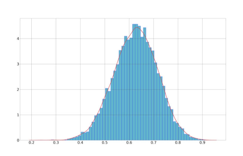
But the average f is not a safe fraction because 50% of the values lie below the average. We seek an optimal f that guarantees as much as possible that no future values lie below it.
Opt f Key Values
       max: 91.33%
   average: 62.58%
       min: 23.57%
Thus, to be safe, we want the minimum f, which is 23.57%.
The Live Trade Signals using a fixed 1% risk per trade
To create a reference from which to compare our proposal, we have computed what would have been four years of trading activity using our Live Signals.
The next figure shows the equity curves resulting from the 10K resamples, corresponding to a 1% dollar risk on each trade and over what would have been approximately one year of activity.
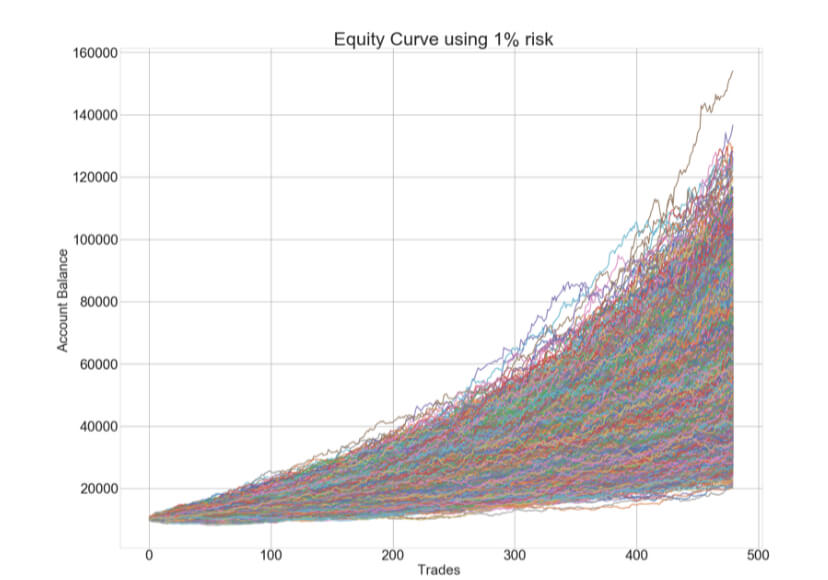
We see that starting with $10,000, the end capital of the equity curves range from $19,967 up to over $140,000, although the average ending capital is $53,122.
      Average ending Capital : 53,122.77
          Max ending Capital : 154,077.50
           Min ending Capital: 19,967.23
From these data, we can also create an interesting statistic to answer the question of how many trades are needed to reach a determined goal. In this case, we present the Trades to reach 10X. The curve results from computing this value on all 10K equity curves and computes the odds relative to the number of trades.
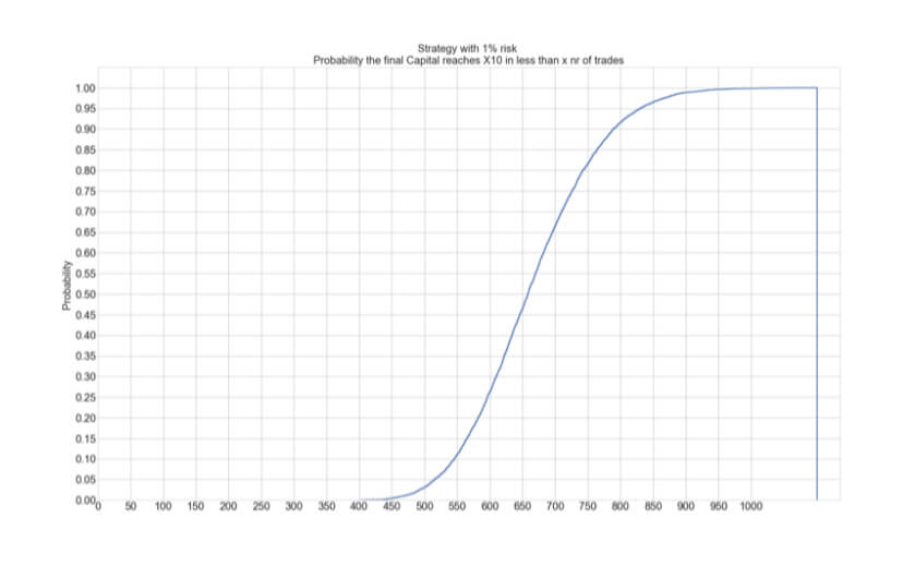
In the case of the 1% risk, we see that the average time to reach 10X, the initial capital is about 650 trades, with a minimum of 400 days and a maximum of 1000 days. Not bad at all. But that can be improved dramatically using a mix of conservative and aggressive position sizing.
The optimal F Positioning Strategy
Using the optimal f positioning strategy, a bold investor will navigate in the turbulent waters of one of these equity curves:
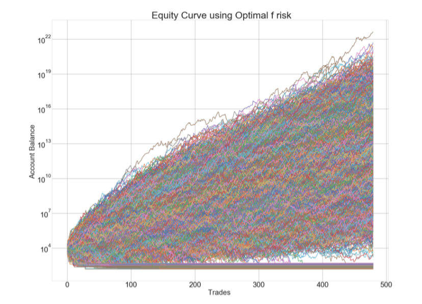
The chart is on a semi-log scale because the range of values is too vast to handle on a linear chart. We see that the y-axis show scientific notation, but do not fret. The number of trailing zeros of the equity corresponds with the last digit is in superscript. For instance, in the previous figure, we see that the ending capital after one year of trades ranges from below $1,000 to a theoretical value with 22 trailing zeros.
The next figure shows the cumulated probability of reaching a certain number of trailing zeros:
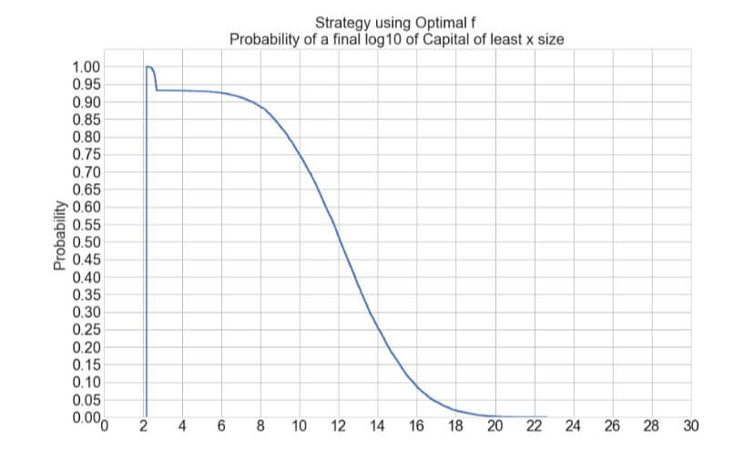
We observe that a small portion of the equity curves end below 4 digits, meaning they are net losers. The following data clarifies this by showing relevant figures:
      Average ending Capital : 517.14 billion
          Max ending Capital : 43,096,478,975,341.38 billion
           Min ending Capital: 153.51
     Capital ending above 517 billion : 55.63 % of the equity curves
     Capital ending above 1 million :  92.51 %
     Capital ending above 100,000 : 92.96 %
     Capital ending below 10,000 :  6.8507 %
     Capital ending below 5,000 :  3.4253 %
And, next, the chart that shows the power of trading using optimal f. The chart shows the time to reach 10X the initial capital,
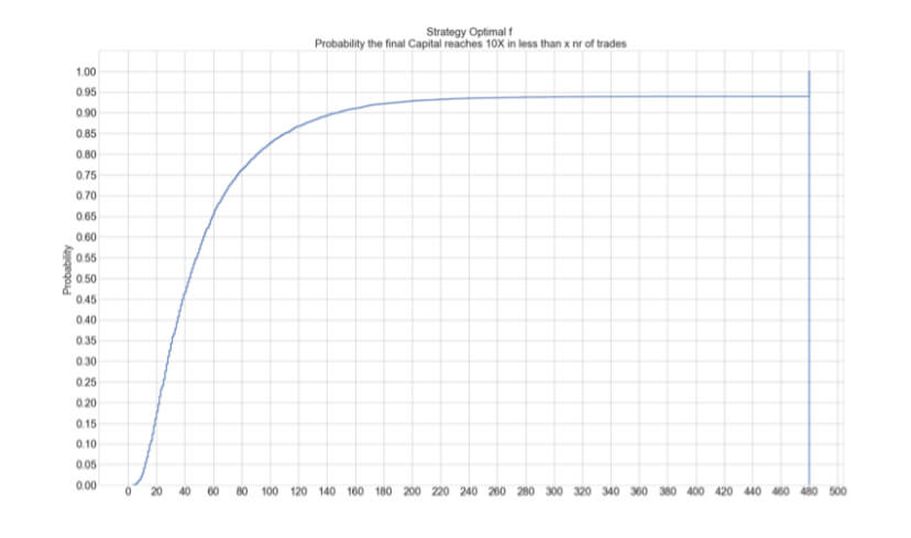
The graph shows that the average time to reach 10X growth (50% probability) went from about 620 days down to 42 days. The same growth achieved in one-tenth of the time!
The Two-tier risk system.
The proposed system aims to profit from the rapid growth of an optimal fraction position sizing while minimizing the risk of blowing up the account. In this video, we will outline the idea and, in the following videos, will present its results and also the optimal requirements to make it work and minimize the risk.
The critical value here is the percentage of times the optimal f ends below 10K in a determined period. Here we will take 80 trades instead of one-year of trading, as this shows a more realistic use in a Two-tier system.
40-trade figures:
    Average ending Capital : 213,793
        Max ending Capital : 5,127 billion
         Min ending Capital: 154
Odds of
             Ending above 46,474    : 51.74 %
             Ending above 1,000,000 : 29.61 %
             Ending above 100,000   : 62.82 %
             Ending below 10,000    : 13.35 %
             Ending below 5,000     : 10.40 %
The key idea is based on the odds of the trading capital ending below the initial 10K value. In the case of sequences of 80 trades, we see that the odds are roughly 13.3%, and the odds of ending below 50% of the original figure is just 10.4%.
That is the risk for the opportunity to have an average of $213,793 ending capital, which is over 21X. The risk/ reward ratio of the proposition is 214/5, which is 43. That means we can be wrong up to 42 times and recover after just one good trading sequence. Our initial proposal is to take 1/4 of the capital to allocate for an opt f positioning strategy.
The Two-tier optimal f proposal
- Take 25% of your current trading balance and use it for the optimal f strategy. Use the rest 75% for 1% risk trades or let it be in cash. (more variations possible)
- Let computations of the optimal f strategy be separated in its own pocket to compute the subsequent trades.
- The account will be rebalanced after a determined goal has been achieved or goes below a predetermined level ( in our case, we will rebalance if the Optf part drops below ¼ of the initial capital on each cycle).
- After rebalancing, a new cycle of 25%-75% allocation begins.
In our next video, we will deal with the results and trade parameters of this combined strategy, as well as our advice on which features are desirable to make this strategy optimal.
Related posts
 Position Sizing Part 1 Drawdown – Why You Keep Blowing Your Account!
 Forex Position Sizing Part 12 – Two Tier Optimal F Part 2
 Forex Trading Algorithms Part 1-Converting Trading Strategy To EA’s & Running Tests On Profitability
 Forex Trading Algorithms Part 5 Elements Of Computer Languages For EA Design!