After completing our series on position size, we would like to summarize what we have learned and make conclusions.
Starting this video series, we have understood that position size is the most crucial factor in trading. On Position Size: The most crucial factor in trading, we learned that deciding the position’s size is not intuitive. In an experiment made by Ralf Vince using forty PHDs with a system with 60 percent winners, only two ended up making money. Thus, if even PHDs couldn’t making money on a profitable strategy, Why do you think you’re going to do it right? You need to follow a set of rules not to fool yourself.
The Golden rules of trading
The trading environment seems simple, but it’s tough. You have total freedom to choose entries, exits, and the size of your trade. Some brokers even offer you up to 500x leverage. But you’re not free from yourself and your psychological weakness, Therefore, you need to set up a set of rules to stop the market to play with you. In “The golden rules of Forex trading” I, II, and III, we propose specific rules it is advisable to follow to succeed in trading. These include never open a position without knowing your dollar risk, defining your profits in terms of reward/risk factors, and limit your losses to less than 1R, a risk unit. We also advise to keep a record of trades and identify your strategy’s basic stats: Average profit, the standard deviation of the profits, and drawdown.
The dark side of the trade
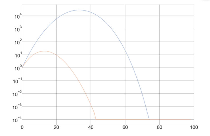
In our video, The Dark Side of Trade, we explain the relation between position size, results, and drawdown, showing that position size plays a vital role in both aspects. In the video, We show that while results grow geometrically ( 100x), drawdown increase arithmetically, 10X. But the lesson here is that the size of the position must be chosen with the drawdown in mind. That is, we should choose a position size so that the max drawdown could be limited to a desirable size.
The Gamblers Fallacy
on Position Size – The Gamblers Fallacy, we explain why it is wise to consider position sizing independently of the previous results. We explain that a new trading result does not usually depend on prior results; thus, modulating the trade size, such as do Martingale systems, is not only useless but dangerous because winning or losing streak ends are unpredictable.
The Advantage!
Even when most retail traders don’t realize it, the “how much” question is the advantage or critical factor to achieve your trading goals because the size of the position defines both the trading results and the risk, or max drawdown, in your trading portfolio. We mention in Position Sizing III- The Advantage that in 1991 the Financial Analyst Journal published a study on the performance of 82 portfolio managers over a 10-year period. The conclusion was that 90% of their portfolio differences were due to “asset allocation,” a nice word for “investment size.”
In this article, we also presented the simplified MCP model to compute the right lots to trade as:
M = C/P, where M is the number of lots, C is the (Cash at) Risk, and P is the Pip distance from entry to stop-loss. The cash will depend on the percent you’re willing to risk and the cash available in your trading account.
Equity Calculation Models
In our next video of this series, Position Size IV – Equity Calculation Models, We explain several models to calculate several simultaneous positions:
- The Core Supply Model, in which you determine the nest trade’s size using the remaining cash as the basis for computing C.
- The Balanced Total Supply Model, in which C is determined by the remaining cash plus all the profits secured by a stop-loss.
- The Total Supply Model, in which the available cash is computed by adding all open position’s gains and losses plus the remaining cash.
- The Boosted Supply Model uses two pockets: the Conservative Money Pocket and the Boosted Monet Pocket.
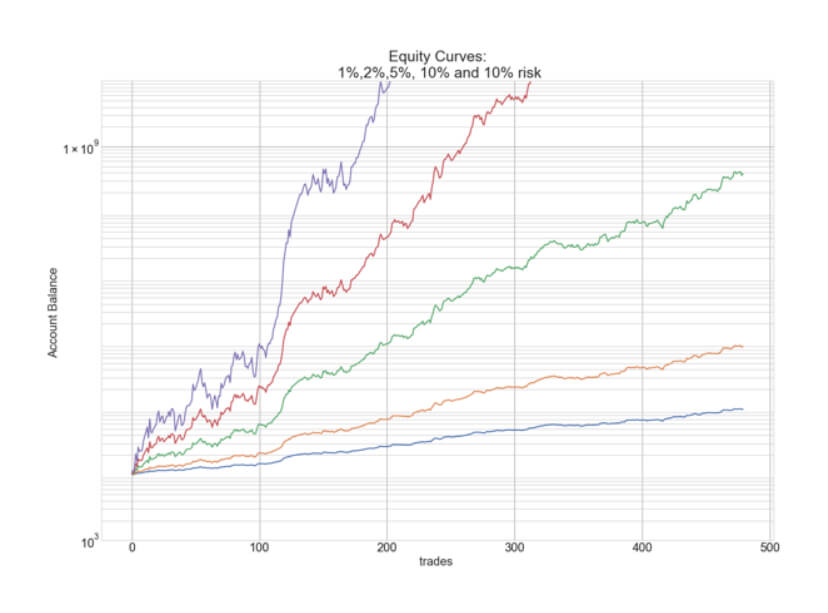
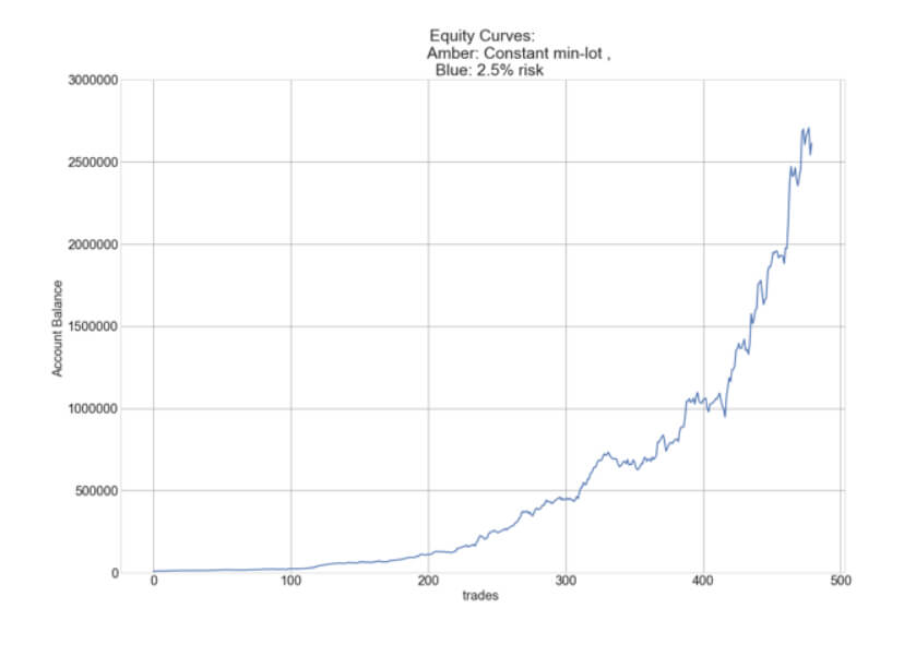
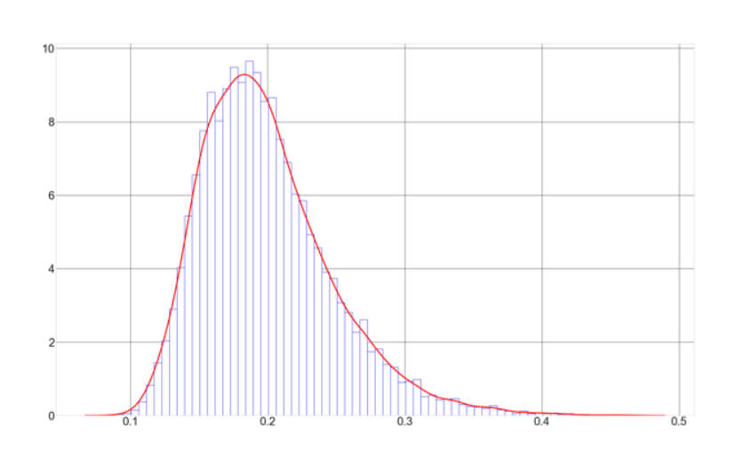
The Percent Risk Model
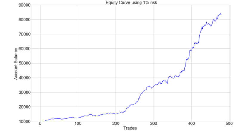
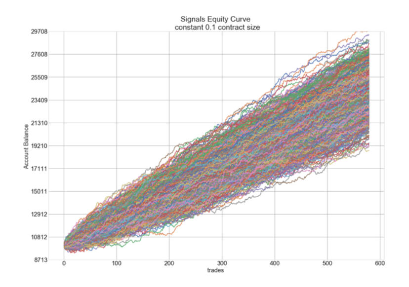
The Percent Risk Mode is the basic position sizing model, barring the constant size model. on Position Sizing Part 5, we analyze how various equity curves arise when using different percent risk sizes and how drawdown changes with risk. Finally, we presented an example using 2.5 percent risk for an average max drawdown of 21 percent.
The Kelly Criterion
Our next station is The Kelly Criterion. The linked article explains how the Kelly Criterion is used to find the optimal bet amount to achieve maximal growth, based on the winner’s percentage and the Reward/risk ratio. The Kelly criterion was meant for constant reward bets, and as such, it cannot be used in trading, but it tells us the limit above which the size of the position increases the risk while decreases the profits. We should be aware of that limit considering that most retail Forex traders trade beyond it and blow out their accounts miserably.
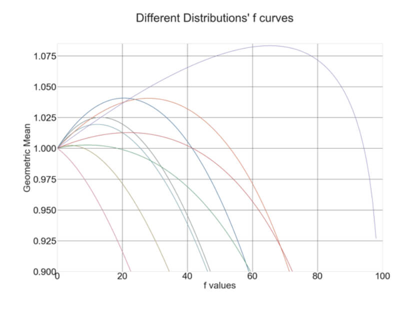
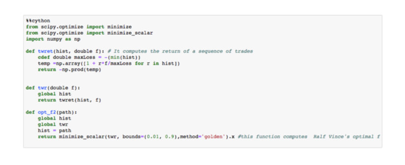
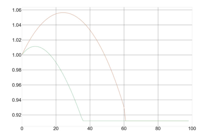
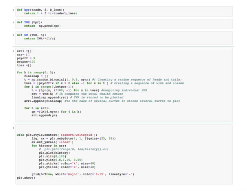
Optimal fixed fraction trading
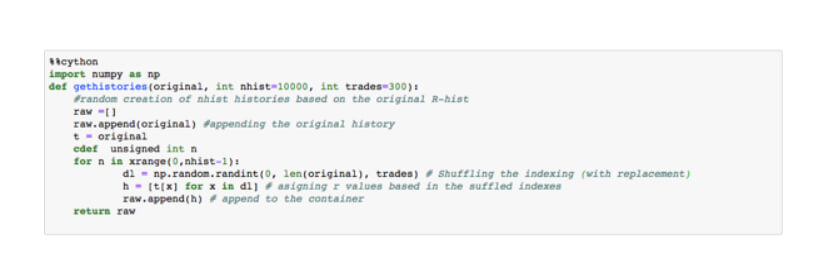
Optimal fixed fraction trading, Optimal f for short, is the adaptation of the Kelly criterion to the financial markets. The optimal f methodology was developed by Ralf Vince. In Position Size VII: Optimal Fixed Fraction Trading, we explain the method and give the Python code to find the Optimal fraction of a stream of trading results. The key idea behind the code is that the optimal fraction is the one that generates the maximal growth factor on a set of trades. That is, Opt F delivers the maximal geometric mean of the trading results.
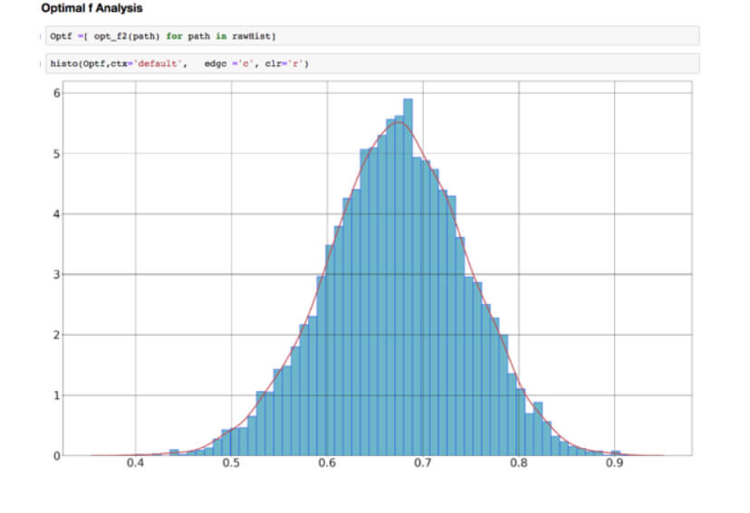
Optimal f properties
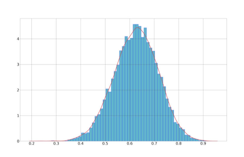
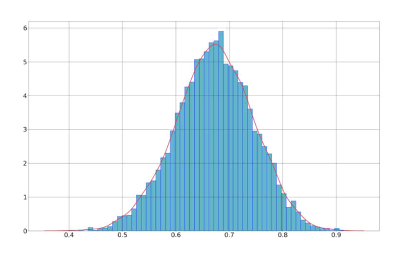
But nothing in life seems easy. Optimal f has dark corners that we should be aware of. In Position size VIII – Optimal F Revisited, we analyze the properties of this positioning methodology. We understood that, due to the trading results’ random nature, we should find a safer way to find the optimal fraction to trade. This article presented a safer way to compute it using Monte Carlo resampling and take the minimum value as optimal f. This way, the risk of ruin is minimized while preserving the strong growth factor Opt f provides.
Market’s money
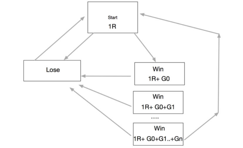
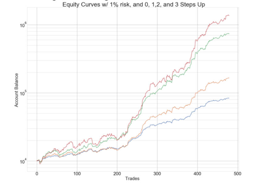
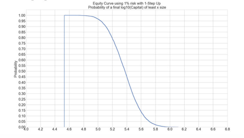
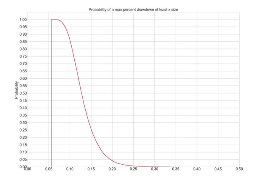
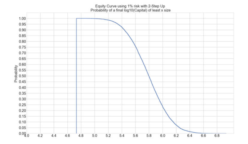
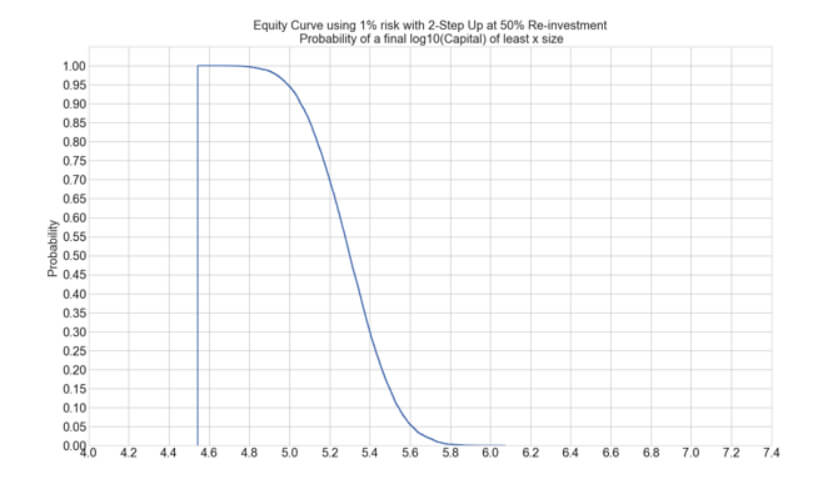
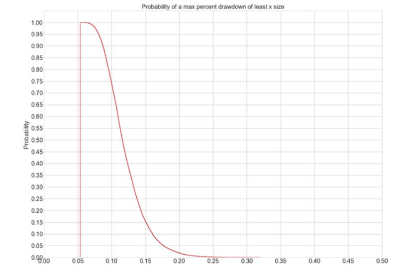
Traders define their recent trading gains as “market’s money. A clever way to profit from the usual winning streaks is to use the market’s money to increase the position size in a planned manner. In Position Sizing IX: Improving the Percent Risk Model-Playing with market’s money,
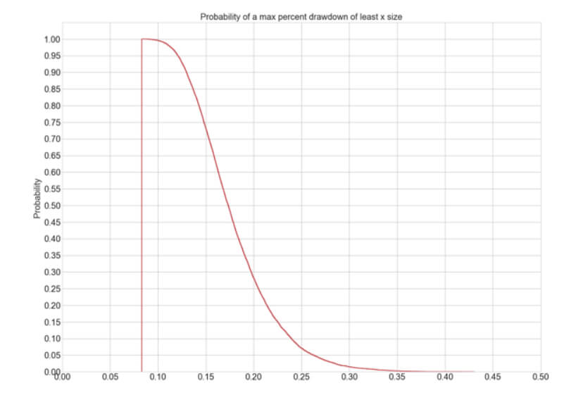
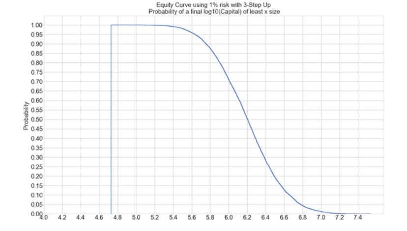
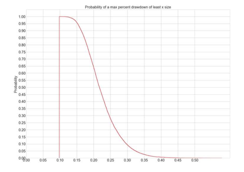
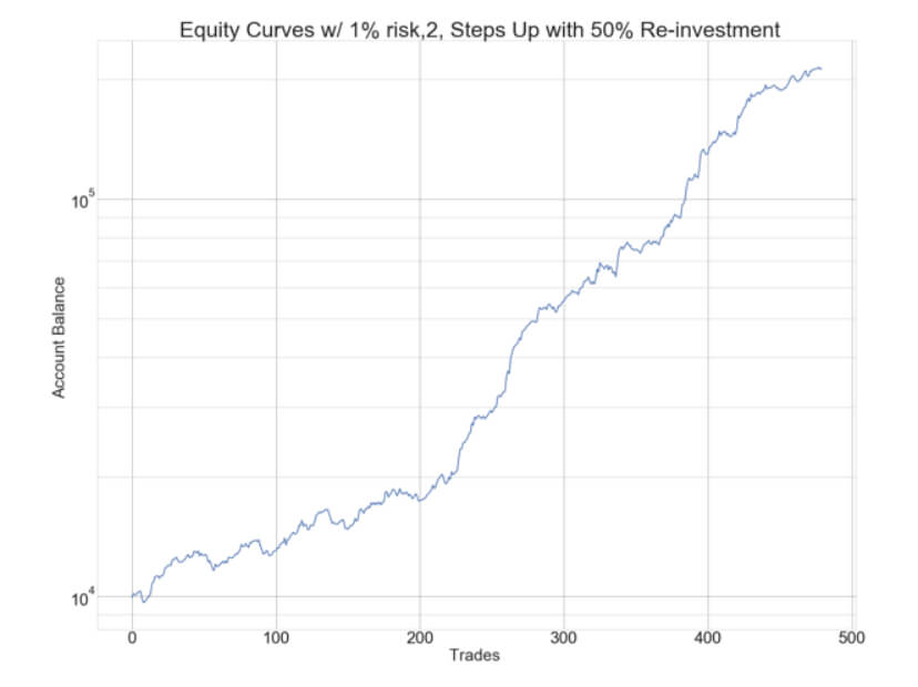
we present the N-Step Up position sizing strategy, an innovative algorithm that adds the gains obtained in previous trades to boost the profits. This way, it could increase the profitability by 10X with a max drawdown increase of roughly 2.8X, from 8.02% to 22.5%. This article analyzes four models: one, two, and three steps with 100% reinvestment and three steps with 50% reinvestment.
Scaling in and out
Our next section, Position sizing X: Scaling-in and scaling-out techniques, is dedicated to scaling in and out methods. Scaling in and out are techniques to increase the position size while maintaining the risk at bay. They work best with trending markets, for instance, the current crypto and gold markets. The main idea is to use the market’s money to add to our current position while trailing our stops.
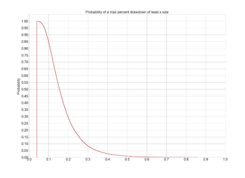
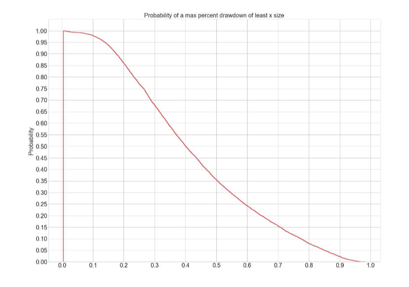
System Quality and Max Position Size
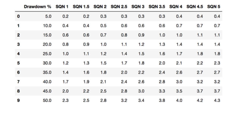
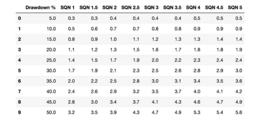
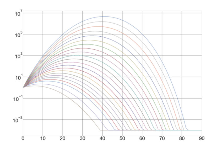
System quality has a profound influence over the risk, and, hence, over the maximum position size, a trader can take. In Position Sizing XI- System Quality and Max Position Size Part I and part II, we presented a study on how the trading strategy’s quality influences the maximum position size a trader should take. To accomplish this, we created nine systems with the same percentage of winners, 50 percent. We used Van K Tharp SQN formula to compute their quality and adjusted the reward to risk on each system to create nine variations with SQN from 1 to 5 in 0.5 steps.
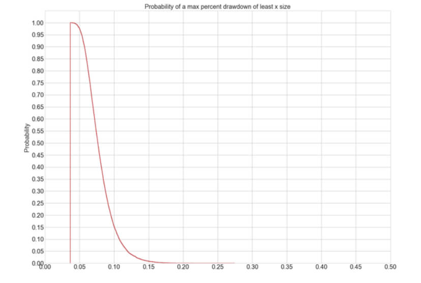
Then, since traders have different risk limits, we defined as ruin, a max drawdown below ten preset levels from 5 to 50 in 5-step.
Our procedure was to create a Monte Carlo resampling of the synthetic results, which simulated 10 thousand years of trading history on each system.
Since a trading strategy or system is a mix between the trading logic and the trader’s discipline and experience, we can estimate that the overall outcome results from the interaction of the logic and the treader. Thus, we can accurately associate a lower SQN with lowing experienced traders and higher SQN to more professional traders. The study’s concussions suggest a limit of 0.5 percent risk on newbies, whereas more experienced traders could boost their trading risk to an overall 4.5%.
Two-tier Optimal f Positioning
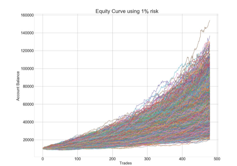
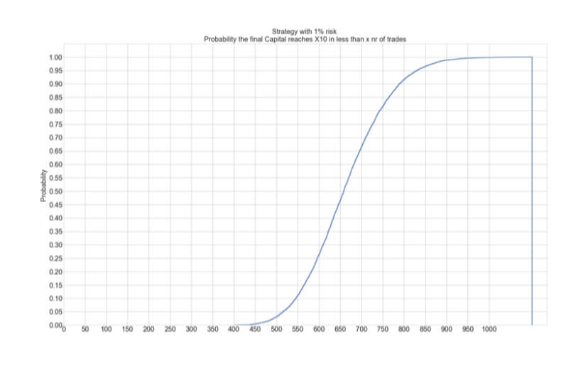
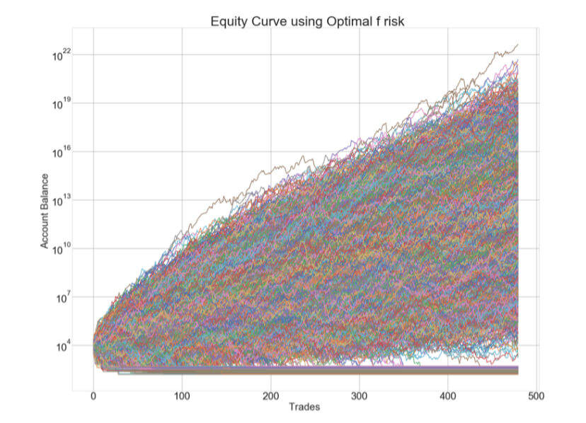
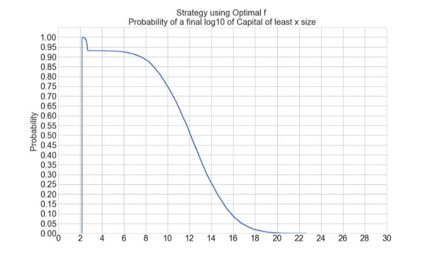
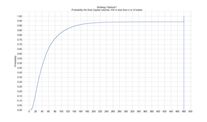
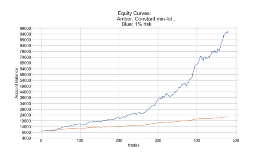
After this journey, we have understood that Using Ralf Vince’s optimal f position sizing method means maximally growing a portfolio. Still, the risk of a 95% drawdown makes it unbearable for any human being. Only non-sentient robots can withstand such heavy drops. In Position sizing XII- Two-tier Optimal f, we analyzed the growth speed of a 1% risk size, and we compare it with the Optimal f. We were interested in the average time to reach a 10X final capital. We saw that on a system with 65.5% winners and a profit factor of 2 ( average Reward/risk ratio of 1.1), using 1 percent risk, it would take650 days ( about two years) on average, whereas, using optimal f sizes, this growth was reached in 42 days, less than one-tenth of the time!.
The two-tier Optimal f positioning method uses the boosted supply model, and is a compromise between maximal growth and risk. The main objectives were to preserve the initial capital while maintaining the Optimal f method’s growth characteristics as much as possible.
The two-tier optimal f creates two pockets in the trading account.
- The first pocket, representing 25% of the total trading capital, will be employed for the optimal f method. The rest, 75%, will use the conservative model of the 1 percent model.
- After a determined goal ( 2X, 5X, 10X, 20X), the account is rebalanced and re-split to begin a new cycle.
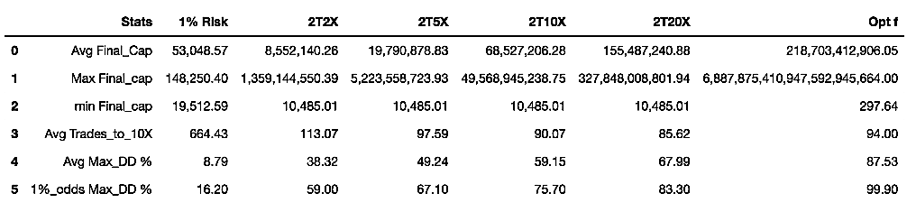
In Position sizing XII- Two-tier Optimal f part II, we presented the Python code to accurately test the approach using Monte Carlo resampling, creating 10,000 years of trading history.
The results obtained proved that this methodology preserved the initial capital. This feat is quite significant because it shows the trader will dispose of unlimited trials without blowing out his account. Since the odds of ending in the lowest possible scenario are very low, there is almost the certainty of extremely fast growths.
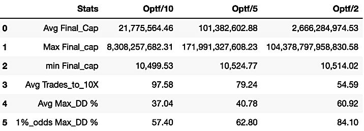
Finally, we also analyzed other mixes in the two-tier model, using Optf / 10, Optf/5, and Optf/2 instead of 1%, with goals of 10X growth to rebalance. These showed extraordinary results as well while preserving the initial capital. B.
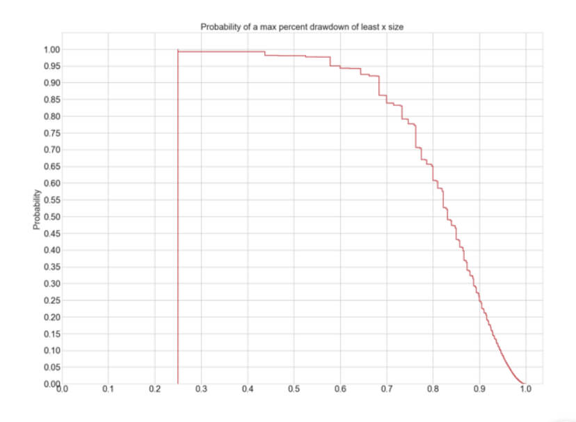
Drawdowns
The trader should also consider the drawdowns involved before deciding which strategy best fit his tastes because, while this methodology lowers it, in some cases, it goes, on average, beyond 60%. We have found that the best balance between growth and risk was the combination of 75% Optf/10 and 25% Optf, which gave an average final capital of $21.775 million with an average drawdown of 37%.
To profit from this methodology, the trader must ensure the long-term profitability of his system. Secondly, he must perform a Monte Carlo analysis to find the lowest optimal f value. Finally, he should create an adequate spreadsheet to follow the plan.
Final words
After reading all this, we hope you know the importance of position sizing for your success goals as a trader.
One caveat: We have left some topics out, such as martingale methods, which many traders use and are the main cause of account blown out. Please adhere to the philosophy that position sizing should be thought of as a tool to reach your goals and handle your risk and drawdowns. As shown in The Dark Side of the trade, position sizing should be separated from the previous trades’ results.