
Position Sizing VII – Optimal Fixed Fraction Trading (I)
In the previous video, we have discussed the virtues and drawbacks of the Kelly Criterion. But, the Kelly Criterion formula is valid for fixed outcomes, such as bets, in which the gambler wins or loses predefined amounts, and the probability of success is known. In this video, we are going to explain Ralf Vince’s Optimal f. Optimal f is Ralf’s way of applying the concept of Optimal Fixed Fraction to the markets.
Investing in the markets generates a sequence of wins and losses. If this sequence has a positive mathematical expectation when using a normalized risk unit, ” […] there exists an optimal fraction between zero and one as a divisor of your biggest loss to bet on each and every event.” (Ralf Vince, The handbook of Portfolio Mathematics).
Many people think that the more you bet, the more you’re going to make. That is true in risk-free investing, but it is evident that if you risk 100% of your capital in a trade and lose, you’re losing all your funds. As we have seen in the previous video, there exists an optimal bet size that creates the highest multiplier for your initial capital. This value is different for strategies with distinct parameters.
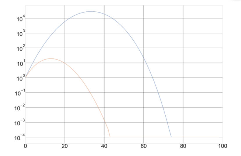
The figure below shows the return curves of two games after 100 bets. The first blue one corresponds to the fair coin toss game with a 2:1 payoff. The amber curve corresponds to a game with 30% winning percent and 4:1 payoff. We can see that the top of the curves representing the optimal fraction to trade is different, as expected.
How to find the optimal f under market conditions
As said, the Kelly Criterion is valid when the size of the payoff and probability of success is known. When it is not, such as in trading, the procedure to find the optimal fraction is making iterations using different bet sizes to determine the historical best value. Ralf Vince proposes to find it using the Geometrical Mean (GM). He calls HPR to the return of a single trade:
HPR = 1 + f *(-trade/biggest loss)
The product of HPRs is what the calls The Total Wealth Return (TWR)
TWR = ∏(1 + f *(-trade/biggest loss)), where ∏ stands for product.
GM = TWR ^(1/n)
Thus, the Geometrical Mean is the n-th root of TWR, Where n is the number of trades. This Geometric Mean is the growth factor of the strategy.
By looping through f values between zero and one we can find the f for which GM is the highest.
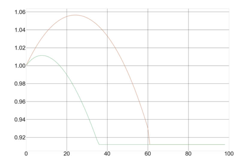
The graph represents the same two games shown above, but depicting the Geometric Mean curves for the different fractions from zero to one. Values below one represent a negative growth factor, meaning the trade size leads to the loss of the capital.
Doing this on Python is straightforward:
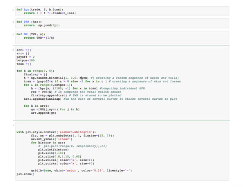
To summarize:
- We take a list of trades of our trading system, with a standard 1 unit position size
- We create a loop from 0 to 100 compute the individual HPR of the trades using the different fractions.
- We compute the HPR for each trade fraction
- We compute its geometric mean (GM)
- We find the optimal f, which is the fraction that delivers the highest GM
Once found, we compute the optimal trade units using the formula
Units = Largest Loss / f.
for example, if our largest loss is $100 and f= 0.2, then Units = $100/0.2 , or $500. This means to trade one unit for every $500 in the cash balance of your trading account.
We see that the optimal fraction is a divisor of your biggest loss that gives you the dollars needed in your account for every unit of trade (lot or contract)
In the next video, we will continue discovering the properties of the optimal f, stay tuned…