Categories
Forex Fibonacci

You’re still using Fibonacci Retracements Incorrectly

You’re still using Fibonacci retracements incorrectly

Like any discipline or field of study, Technical Analysis goes through changes. Old theories and approaches are rigorously utilized and tested, new ideas are studied, and advancements in the field occur. And, like any discipline or study, it takes a while for people to adapt to the new way of doing things. There is a shocking amount of updated theory and application in Technical Analysis that has yet to make its way down to the retail trader and investor – some of it is almost 25+ years old! One of the updates to old application and practice is how we use a tool known as a Fibonacci retracement. For many years, the method has been to draw a retracement from one extreme swing to the next (from swing high to swing low or swing low to swing high). In practice, there are a few incidents where this may work out just fine, but the new and better way shows how much more accurate and useful the update has been.


Old vs. New

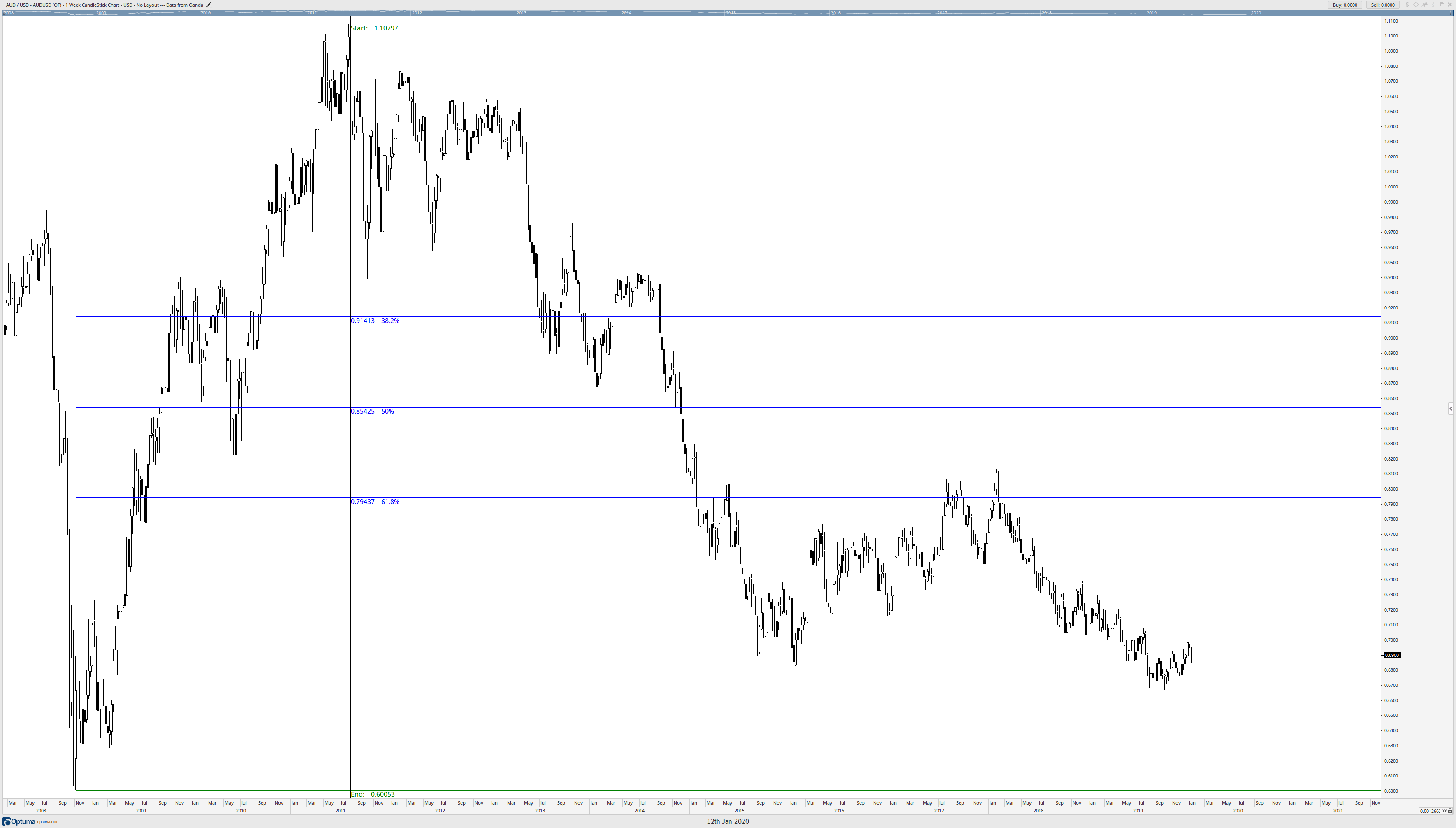
I want to start off right away by showing you the difference between the old and new methods – I reference the new approach as the Brown Method. The AUDUSD Weekly chart below shows the old way of drawing Fibonacci retracements. With the old process, the Fibonacci retracement is drawn from the extreme swing high on the week of August 5th, 2011, to the extreme swing low on the week of October 31st, 2008. The vertical line delineates the starting point of the retracement, and no data to the left of that vertical line should be used to determine the efficacy of the retracement. It is only the data after the vertical line that is important and relevant.

Fibonacci Retracement: Incorrect

Now, contrast the image above with the new Brown method below.

Fibonacci Retracement: Correct

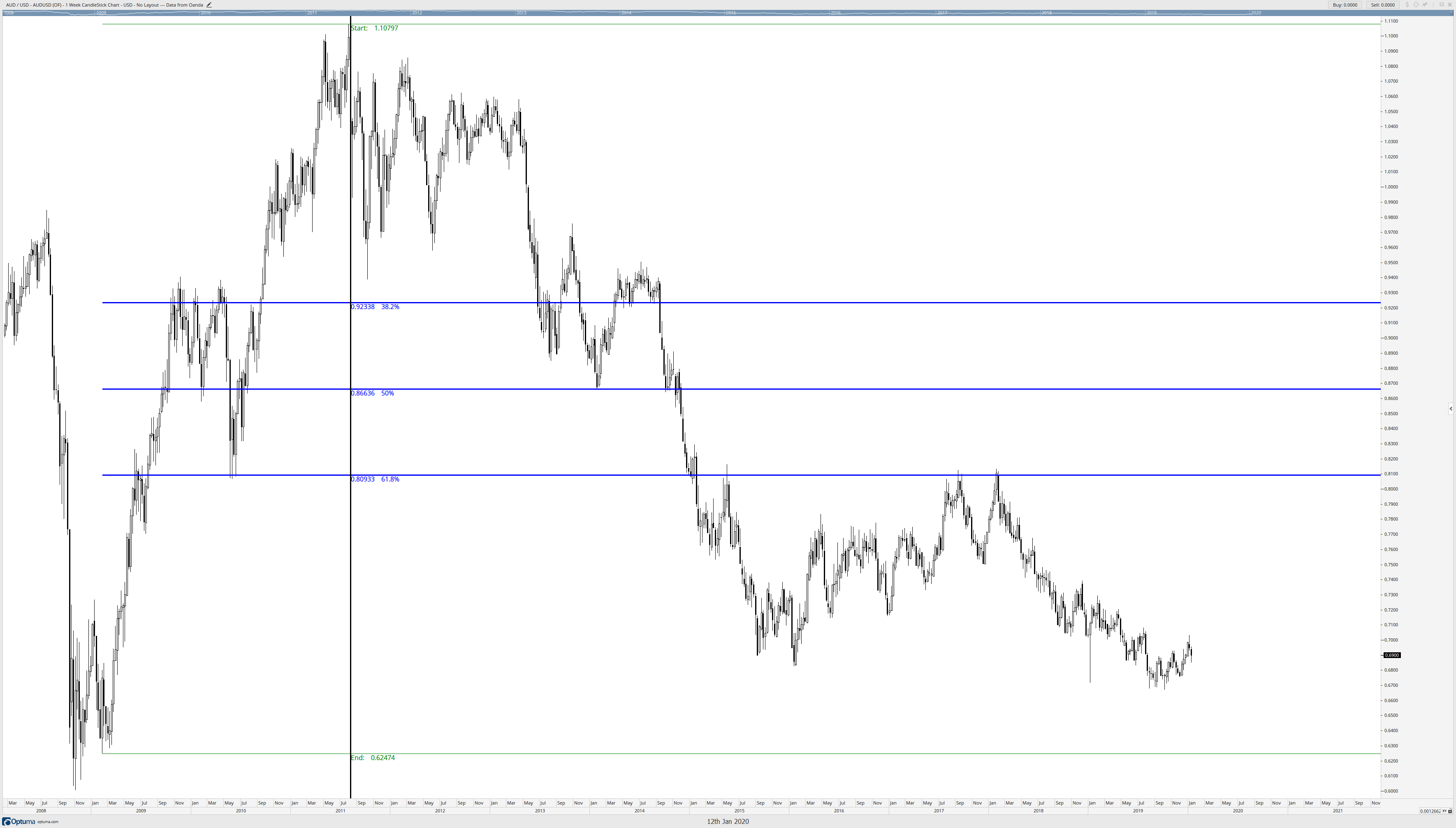
You will observe how much more accurate the Fibonacci retracement levels are on the Brown Method vs. the old method. What changed? Observe the swing low retracement on both charts – they are different. They both start at the same level, but the retracement end for the Brown method is drawn to the swing low on the week of February 6th, 2009. But why? Why do you draw to a seemingly random or ‘off’ swing and not the extreme? The reason for this is based on the writings of W.D. Gann.


The Brown Method

I call this new Fibonacci retracement method, the Brown Method, after Connie Brown. It is Connie Brown who discovered this new theory and wrote about it in her 2008 book, Fibonacci Analysis. It is not a very large book, under 200 pages, but it is one of the single most important works in Technical Analysis of the past 15-years. Her discoveries of how confluence zones of Fibonacci retracements dictate the normal rhythm and pulse of the market are truly groundbreaking. But to the first question of why I did not draw the retracement to the extreme low? Connie Brown points out that W.D. Gann made the point that the end of a trend is not established by the extreme high or low – it is the secondary high/low that confirms the change in trend (sometimes known as the confirmation swing). This makes sense because the extreme is very rarely the level where the participants in a market agree that a trend is finished.

So how do we identify what swing to use? How did I identify what candlestick was the confirmation swing low on the weekly AUDUSD chart? Again, this goes back to Brown – but this information is from her penultimate work (her magnum opus in my opinion), The 32nd Jewel. The first chapter of her massive book (it weighs about eight lbs., is three inches thick and nearly 1100 pages long) addresses some of the problems students of hers have had with the application of her updated Fibonacci retracement method. To identify the correct swing to use, we look for the strongest bar. Let’s take a ‘zoomed’ in look at the swing low used on the AUDUSD weekly chart above.

Brown Method: Confirmation higher swing low

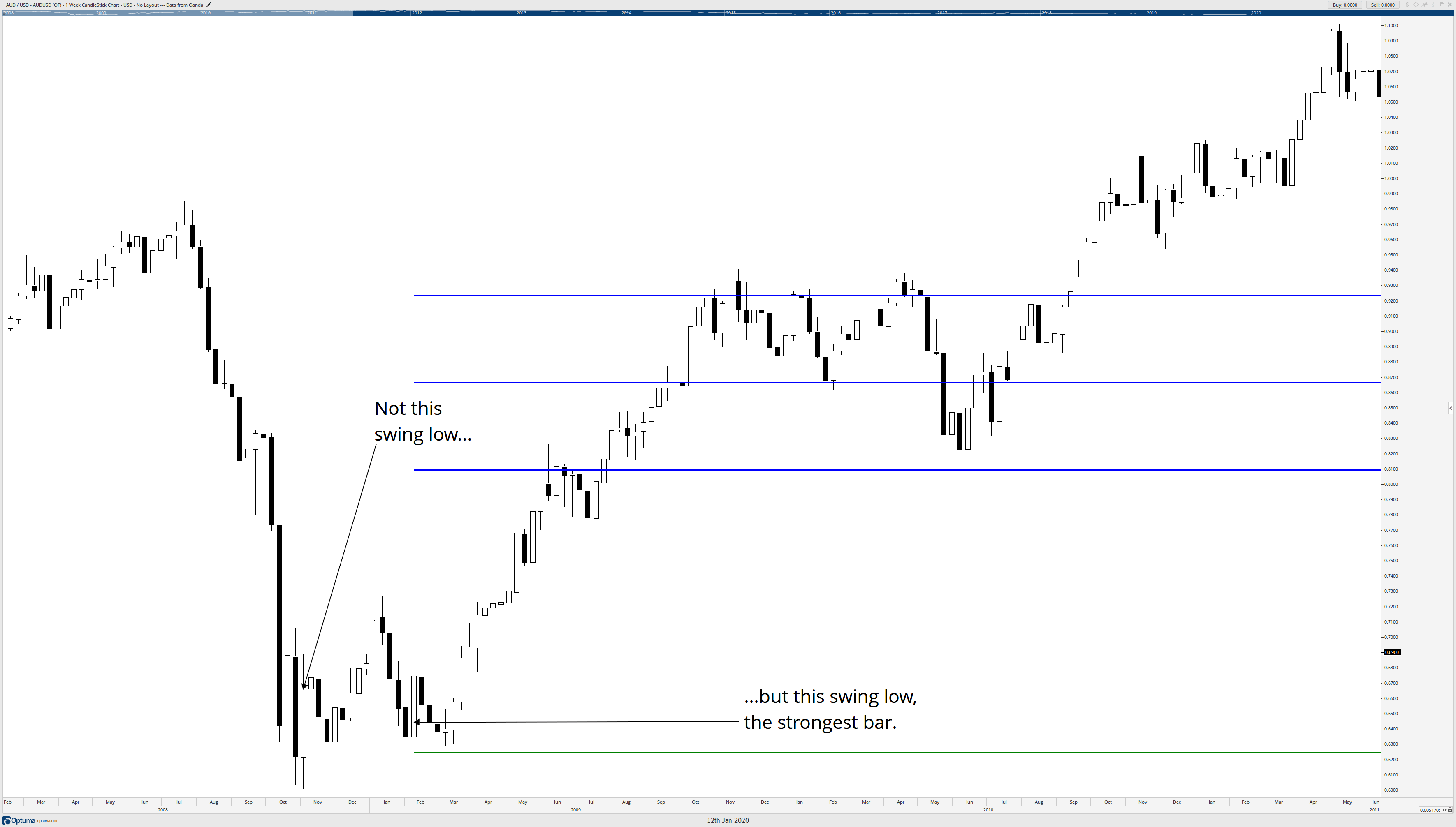
It will take you some practice to find the swing bar (also, gaps are used, but that is for another article) that would be considered the ‘strong bar.’ What constitutes a strong bar? That can be somewhat subjective, but look at the candlestick that I’ve identified as the strong bar compared to the candlesticks before it and around it. Why did I pick this candlestick? First, it is a bullish engulfing candlestick on the weekly chart. Second, that candlestick rejected any further downside pressure after a consecutive four week period of weekly candlestick closes below the open. Third, the open and low of the candlestick created the support zone for the next five weeks. In a nutshell, the candlestick is massive, its sentiment overwhelmingly one-directional, and the lows of that candlestick were respected. That candlestick was the confirmation swing low because it confirmed the end to lower prices and was the most substantial candlestick before the new uptrend occurred.


Side note: Connie Brown also said to look for gaps in the price action as areas to draw the confirmation swing. Finding gaps is a much easier process when looking at traditional markets like the stock market. Forex data can vary from broker to broker as some data providers show gaps, and others do not.


The following articles will go into further detail on how to implement more of the Brown Method. I believe that what you will read and learn will be one of the ‘wow’ moments you experience in the study of Technical Analysis. To say that what Connie Brown has discovered is truly amazing is an understatement when we learn about the confluence of Fibonacci zones and how they create the natural price zones that an instrument swings to, it is a truly eye-opening experience.


Sources:

Brown, C. (2010). Fibonacci Analysis: Fibonacci Analysis. Hoboken: Wiley.

Brown, C. (2019). The Thirty-Second Jewell: Thirty Years Behind Market Charts From Price To W.D. Gann Time Cycles. Tyton, NC: Aerodynamic Investments Inc.

Categories
Elliott Wave Guide Forex Elliott Wave

Essential Elliott Wave Theory Guideline

Recently, we ended the series that presents the basic concepts of the Elliott Wave Theory. In this guideline, we disclose the contents developed.

  1. Fundamentals of Elliott Wave Theory. Divided into three parts, we introduce the basic concepts of the wave principle.
    1. Wave principle and the five-waves structure.
    2. Motive waves, corrective waves, and cycles.
    3. Degrees and labeling.
  2. Planning the First Wave Analysis. In this two-parts chapter, we explain the necessary steps to analyze using the Elliott wave principle.
    1. Setting charts and the identification process.
    2. Proportionality and the relationship between price and time.
  3. Impulsive Waves Construction. This section offers the key concepts to understand the nature of impulsive waves.
    1. Nature of impulsive waves and the alternation principle.
    2. The channeling process.
    3. Extensions.
    4. Leading and Ending Diagonal.
  4. Corrective Waves Construction. Elliott, in his Treatise, spent a large part of time describing corrective waves. In this section, we present different corrective formations.
    1. Nature of corrective waves and alternation.
    2. Zig-zag pattern.
    3. Flat pattern.
    4. Triangles.
    5. Complex corrective waves.
  5. Elliott Wave Theory and Fibonacci. In this one-part article unfolds the keys to use Fibonacci retracement and expansion tools.
  6. Trading the Elliott Wave Principle. We end the cycle of the Elliott wave theory with the five-part guidelines.
    1. Wave three structure trading setup.
    2. Wave five and ending diagonal trading setup.
    3. Zig-zag pattern trading setup.
    4. Flat pattern trading setup.
    5. Triangle formation trading setup.
Categories
Forex Elliott Wave

Traders’ Guide to the Elliott Wave Theory

The Elliott wave principle has its origin in the early 1930’s decade. The introduction of the wave concept was published in 1934 by R.N. Elliott in his work “The Wave Principle.”

The Wave Principle

In Elliott’s treatise, the author indicates that financial markets as a socio-economic activity hold a specific structure composed of five waves. In his model, Elliott teaches us that waves 1, 3, and 5, move following the direction of the dominant trend. On the contrary, waves 2 and 4 develop an opposite movement to the primary trend.

Parts of the Cycle

The Elliott wave cycle has two components; these components are an impulsive wave and a corrective wave.

As said before, an impulsive sequence holds five waves; and a corrective wave contains three segments. In consequence, a complete cycle has eight waves.

The next figure unveils a complete Elliott wave cycle.

The Analysis Process

When R.N. Elliott developed its theory, he defined a specific terminology to maintain the order in the analysis process. The author established a series of degrees that must be considered in relative terms about price and time.

The next table illustrates the different degrees defined by Elliott.

The analysis process starts with the relevant highs and lows identification in a larger timeframe. After this, we proceed to study the prices’ sequence; to aid to do this step, we examine the proportionality and the relation between price and time. The next chart illustrates the relationship between price and time.


The next stage is to identify impulsive waves. The basic guidelines of motive waves are:

  1. It has five consecutive segments building a trend.
  2. Three segments move in the same direction.
  3. Wave three never is the shortest.
  4. Wave two never ends below the origin of wave one.
  5. When an impulsive movement finishes, it starts a corrective move of the same degree.

Alternation is a key concept of the wave principle. We observe the motive and corrective waves alternate one with another.

We observe the alternation in:

  • Distance.
  • Time.
  • Retracement.
  • Complexity.

The following EURAUD charts illustrate the concept of an alternation.

Categories
Forex Elliott Wave

Corrective Waves Construction – Part 2

R.N. Elliott, in his work “The Wave Principle” described the zig-zag structure as a corrective pattern. In this educational article, we will unfold the zig-zag formation.

The basics

The zig-zag pattern contains three waves in a higher degree, and follow a 5-3-5 sequence in its lower degree. This order means that the first leg (A) has five internal waves; the wave (B) has three segments. Finally, wave (C) is formed by five waves. The following picture shows the formation of a zig-zag pattern.


Zig-zag variations

A zig-zag pattern could develop some variations as a normal, truncated, and extended. The following chart represents the different variations of the zig-zag structure.

Consider as a key to classify what kind of zig-zag structure is running, each segment of the corrective wave must follow the 5-3-5- sequence, and the extension of wave C.


Zig-zag patterns: Channeling

Another tool to identify the type of zig-zag pattern is the use of channels. Channeling allows us to identify the potential movement of a zig-zag formation.

Channeling is developed in the same way as motive waves. In this case, we must connect the end of the last motive wave with the end of wave B and project the parallel line at the end of wave A.

In the next figure, we observe the difference between a normal and a truncated zig-zag not necessarily surpass the base-line of the channel. The main difference is that in a normal zig-zag, the wave C projection could be at least 2/3 of wave A.

In the truncated zig-zag, the wave C projection is between 1/3 and less than 2/3 of wave A.

On the extended zig-zag pattern case; the sequence could be indicative of a complex corrective sequence formation.


The S&P 500 weekly chart shows a zig-zag pattern. The bearish sequence started in October 2007 when the price reached at 1,576.1 pts. The corrective move ended on March 2009 at 666.8 pts. In some cases, the line chart could be helpful to visualize each segment of a wave. In this example, we observe in the line chart how the structure accomplishes the 5-3-5 sequence.


Categories
Forex Elliott Wave

Corrective Waves Construction – Part 1

Corrections are formations that occur after each impulse. As we have seen before, corrective waves have three segments. In this article, we will see the main characteristics of the corrective waves.

Nature of the corrective waves

Generally, corrective waves are more challenging to identify than impulsive waves due to their variations. Elliott spent a large part of his time describing the different types of corrections. The author, in his Treatise, explains that “a corrective wave in progress is complicated to predict accurately between its pattern and extent.

Corrections are characterized by having three waves, except triangles that have five internal segments. Some factors that can influence the form of correction are time, speed, the extent of the previous movement, etc.

In the following figure, we observe the formation of the basic corrective structures.


Corrective waves formation

If the price action does not allow all the rules of formation of an impulsive wave to be verified, then the market is developing a corrective structure.

The most straightforward corrective structures are:
– Zig-zag, this formation has a 5-3-5 sequence.
– Flat, whose internal structure has a 3-3-5 configuration.
– Triangles, these formations develop in a sequence 3-3-3-3-3.

There are also corrective structures that are a combination of two or three simple corrective patterns. These formations are known as double three and triple three.

Alternation in the corrective waves

Just as impulsive waves alternate, corrective waves do too. In simple terms, Elliott points out that if wave two is a simple structure, wave four will be complex and vice versa. In the following figure, we observe how the corrective waves alternate in complexity.


Corrective waves can also alternate in the strength level. That is, a correction can be ordinary or strong. In the following chart, we observe the ideal model of the strength level in a corrective structure.


Categories
Forex Elliott Wave

Impulsive Waves Construction – Part 3

An extension is an essential feature of an impulsive movement. In this article, we will see what the characteristic of this type of movement is.

Extensions

An extension is a movement that characterizes the longest wave of an impulsive wave. This movement allows us to differentiate between an impulse and a correction. An extension may appear in waves 1, 3, or 5, but it will never appear in more than one wave. In the following figure, we see the extended wave of “blue” degree and the “black” grade wave corresponds to the upper degree structure.


Extensions of extensions

As in the previous case, extensions can have internal extensions. The rules for this scenario are the same as in the case of simple extensions.


The following figure corresponds to the Dow Jones Industrial Average (DJI) in the semilog scale. The chart shows the impulsive wave that begins with the October 1987 low at 1,616.2 pts., and concludes on October 2007 when DJI touched the 14,198.1 pts. The cycle ended when DJI made a new low in 2009, reaching the 6,470 pts.

Dow Jones chart shows that the third wave of blue degree is the extended wave. Additionally, the third wave of the black degree is the extension of the extension in the bullish cycle.


Categories
Forex Elliott Wave

Impulsive Waves Construction – Part 2

A useful tool for motive wave analysis is the use of channels. In this article, we will review how to use channels to identify motive waves.

Channeling process

A channel is a technical figure that is formed by three points. In Elliott wave theory, channels allow us to identify the potential objective of waves 3 and 5, with “dramatic precision.”

R.N. Elliott, in his work “The Wave Principle” tells us that a channel cannot be drawn if wave two has not ended. Once this wave is complete, we can trace the first channel by connecting a line from the origin of the first impulse to the end of the second wave. Then, a parallel line is projected at the end of the first wave. The following figure shows the process.


Once the third wave is completed, the same process is repeated, this time, we connect the end of wave 1 and 3, and we make the projection at the end of wave 2. This channel will give us an approximation of the end of wave 4. To estimate the end of the fourth wave, we must consider that it should never be more profound than wave 3. The following figure shows this channeling process.


Finally, once the fourth wave is finished, we draw the baseline of the channel linking the ends of waves 2 and 4 and project the parallel line at the end of the third wave. This channel will give us as a possible end of the fifth wave.


The following Silver daily chart shows that the precious metal is completed a sequence of three waves. Currently, the commodity is running in a wave 4 with a potential target at the $17.5 zone.


Categories
Forex Elliott Wave

Impulsive Waves Construction – Part 1

Previously we presented an ideal model of motive waves; however, the real market is not exactly perfect. In this educational article, we will develop the principles of impulsive waves.

The nature of impulsive waves

Before we begin to identify impulsive waves, we must consider the following rules that compose it:

  1. It must have five consecutive segments, or waves, that develop a trend.
  2. Three of these five waves must move in the same direction; this can be bullish or bearish.
  3. After the initial wave, a shorter sequence must be developed in the opposite direction of the first movement. This movement should never be greater than the advance of the first wave.
  4. The third wave must be larger than the second movement.
  5. After the third impulsive movement, a similar sequence to the second wave should be developed. However, the third segment trend must prevail over the fourth.
  6. The fifth wave, in most cases, will be more extense than the fourth movement. If the fifth wave is smaller than the fourth wave, this is called a “failure.”
  7. When comparing the lengths of waves 1, 3, and 5, the third wave does not necessarily have to be the longest. However, it should not be the shortest.

If one of these rules is not followed, then the movement is not an impulse, the structure corresponds to a corrective sequence.

The alternation principle

Elliott defines alternation as a law of nature, as the day and night alternates, the movements of a market also alternate. The alternation principle establishes that when two waves of the same degree are compared, they are different from each other.

We observe the alternation in:

  • The distance that price travels.
  • The duration of each wave.
  • The retracement of the depth of each impulse (waves 2 and 4).
  • The complexity of each wave, that is, the number of internal waves that compose it.

The following daily chart corresponds to the EURAUD cross. In the chart, we observe the alternation in price and time. The first bullish movement began on August 21, 1997, at 1.42014, this wave was developed on 118 days and increased 2,919 pips or 20.55%. Wave 3 surged on 131 days and reported an increase of 19.83% or 3,121.6 pips. Finally, the fifth wave grew in 81 days, advancing 3,059.5 pips, or 17.44%, reaching the high at 2,05983 on October 06, 1998.


In the following EURAUD daily chart, we recognize the alternation in the retracement. From wave 2, we observed that the retrace of wave 1, was developed for 44 days, and the cross plunged 8.05% or 1,377.9 pips. Finally, wave 4 fell 1,334.1 pips (7.07%) of wave 3 in 36 days.


Categories
Forex Elliott Wave

Planning your First Wave Analysis – Part 2

In a previous post, we talked about the ideal structure of an impulsive and corrective wave. Also, we discuss the starting point of the study of a market. In this opportunity, we will deepen the steps to identify a wave.


Watching the waves


Before continuing, we must consider the concept of “wave.” A wave is a defined movement of the market, which is reflected in a price variation. Depending on the price action, the change may have a higher or slower speed, but it will never be perfectly horizontal or vertical.

Depending on the sequence of a group of waves, the market may develop an impulsive or a corrective wave structure. An “impulsive wave” is made up of five waves with a relationship of the same degree. On the other hand, a “corrective wave” is composed of a set of three waves. The following figure shows an ideal impulsive and corrective wave.


Wave proportionality

Once we define the start point and the timeframe of the market study, we must consider that waves should have specified “proportionality.” Consider that some Elliott structures could not be easily visible by simple observation. For this reason, we must be flexible in terms of the selection of the timeframe to analyze. Remember that the same timeframe will not necessarily useful to examine all markets. Elliott, in his “Treatise,” reminds us that in markets with low volatility, the weekly chart may be more fit than the daily chart.


Price and time relationship

In a sequential movement, the price action is developed following the relation between price and time. On the following chart, we observe the Financial Select Index ETF (AMEX: XLF) on a weekly timeframe. In the example, we note that the sequence starts in the March 2009 low at $ 4.47, and ends when XLF reached the February 2011 high at $ 13.90. After this top, XLF developed a retrace in February 2011, which led to a higher low at $ 10.02.


In this example, there is a similarity in the advance and retracement of the price with the time. In summary, the movement of two consecutive waves of the same degree cannot be less than one-third (1/3) of the greater in terms of price and time.

Categories
Forex Elliott Wave

Planning the First Wave Analysis – Part 1

Before to start to analyze any market, it’s necessary to set-up the chart earlier to begin to identify motive and corrective waves. In this article, we will learn how to start to analyze the market applying the Elliott Wave Theory.


Setting-up the first chart

The first step consists of choosing the market to be studied, and then select a starting point for the analysis. Once we decided the market of interest and the inception point, in a monthly chart, we will identify the highs and lows of the asset in the order of appearance. After that, we must establish the relevant date and price of every segment.

As an example, the following chart corresponds to the DAX futures in a monthly timeframe. As you can notice, there are identified the “relevant” highs and lows from March 2000 until the present.

Once we defined the starting point,  we will begin the analysis by moving our timeframe from higher to lower. In means, from monthly to daily timeframe, and even to an hourly chart. However, this could demand you extra time to update the analysis.

The identification process

When the identification is complete, we must distinguish the start and end of each wave. From our example, we will start from the March 2009 low at 3,588.5 pts, until the January 2019 high at 13,181.5 pts.

The same process must be realized in the weekly and daily timeframe. As you can notice, we still do not begin to talk about motive and corrective waves. The reason is that the first step is to learn to recognize the movement under study.

As was discussed in the previous article, we will use labels to identify each wave. In our example of the FDAX monthly chart is as follows.


Summarizing, the monthly chart of the FDAX shows a bullish sequence which currently should be developing a wave ((5)). As we learned, waves ((1)), ((3)), and ((5)) moves in the bullish trend direction; it is a motive wave. The waves ((2)), and ((4)) retraces the main trend movement, or in other words, these waves are corrective of the principal trend.

Categories
Forex Elliott Wave

Fundamentals of Elliott Wave Theory – Part 3

Until now, we have defined two kinds of waves, motive and corrective. In this article, we will introduce the concept of “degree,” which will help us in the process of waves identification.

The concept of degree

Elliott defined a series of “degrees” to maintain a hierarchical waves order. This order is based mainly on the relationship that the wave develops over time. In other words, while higher is the time elapsed in the wave formation, greater will be the wave degree.

The term “degree” must be considered in relative terms about the price and time relationship. It should not be considered strictly according to the duration, for example, a day, a week, or a month.

The blue box shows a bullish impulsive wave developed over126 days which attained a 25.95% advance. This wave started from the low of December 26, 2018, when the price found support at 2,346.6 pts and ended on May 1, 2019, when it hit the top at 2,954.4 pts. If we remember the basic structure of a wave, we can see that the upward movement was developed in five waves.

In the red box, we observe a corrective wave sequence disclosed in three waves. This retracement began on May 1 and ended on June 3, 2019, when SPX plunged to 2,728.8 pts. The bearish move unfolded over 33 days and eased 7.67%.


R.N. Elliott, in his work “The Wave Principle” defined a series of degrees, with specific terminology and it’s as follows:

  • Grand Super Cycle.
  • Super Cycle.
  • Cycle.
  • Primary.
  • Intermediate.
  • Minor.
  • Minute.
  • Minuette.
  • Sub-Minuette.

However, Prechter & Frost, in “Elliott Wave Principle” added six degrees:

  • Supermillennium.
  • Millennium.
  • Submillennium.
  • Micro.
  • Submicro.
  • Miniscule.

Despite the wide-spread degrees, Hamilton Bolton says that the most common degrees used are Minor, Intermediate, and Primary.

Wave Labeling

Labels are useful to keep the order in the wave analysis. It’s necessary to assign a symbol on each wave of each wave that is studied. In the Elliott Wave Theory there is a set of labels for each degree as follows:

The wave labels are essential to understand the current market position and will allow us to respond to the question “where goes the market?”.

The following chart corresponds to the application of waves labeling. In this case, the SPX daily chart developed a complete cycle of Intermediate degree.


Categories
Forex Elliott Wave

Fundamentals of Elliott Wave Theory – Part 2

Waves develop in two classes, impulses and corrections. Impulsive movements are characterized by having a five-wave structure. Corrective waves, on the other hand, growth creating a three-wave structure. In this article, we will introduce the concept of motive waves, corrective waves, and cycles.

Motive waves

Motive waves receive this denomination because they create movement, or “impulse” to the price action, as it follows a trend. In the following figure examining the case of a bull market, waves 1, 3 and 5, are impulsive waves. This structure is analogous for a bear market.


Corrective waves

Corrective waves, as the name implies, are characterized by pushing back the price of the dominant trend. From the previous figure, waves 2 and 4 correspond to the corrective waves.

Cycle concept

As we have seen previously, a wave is composed of five waves, and a complete cycle is composed of eight waves, an impulsive part and a corrective part. For convenience in the identification process, we will label motive waves with numbers and corrective waves with letters. Later we will see the usefulness of wave identification to understand the stage in which the market under study is.


When an eight-wave cycle is completed, a new cycle of the same degree begins, as shown in the following figure. This formation generates a five waves sequence of a higher degree. At the moment, you should not be worried about the identification symbols. Elliott defined the labels and should be understood as a tool to help in the study, and not an objective in itself.


Recognizing this structure is essential to understanding the nature of the wave theory.

Categories
Forex Elliott Wave

Fundamentals of Elliott Wave Theory – Part 1

Ralph Nelson Elliott developed the Wave Theory in the 1930s. Elliott discovered that prices followed a sequence of repetitive patterns in form, but not in time and amplitude. He called these patterns “waves,” he also recognized that each movement was composed of five waves.

The Elliott Wave Theory is not a trading system nor a forecasting tool, but, rather, a description of market behavior. In this sense, Elliott waves enable us to understand the current price position and the scenarios that can be anticipated from it. In our first Elliott’s wave theory article, we will review its history and its underlying principles.

Nature and waves

In 1934, R.N. Elliott published his work “The Wave Principle.” It is this treatise, as he calls it, explains the basics of wave theory. In this work, Elliott explains that everything in nature is governed by a law which its causes could be unknown. However, when the law is known, forecasts can be made, regardless of whether or not the reasons that originated it are known. Both nature and universe, some phenomena are repetitive and can be predicted; for example, the lunar phases, the year seasons, the tides, and so on.

Human interactions are part of nature and are no exception in wave theory. The most common socio-economic activity is realized in the financial markets. Elliott remembers us that “there is no socio-economic activity in which so many resources have been allocated and with neither successful results as financial markets.” In this context, wave theory allows us to have an understanding of the current state of financial markets and their possible next path.

The five-wave structure

According to R.N. Elliott, the financial markets as a socio-economic activity hold a specific structure composed of five waves. These waves move in the direction of the dominant trend and are identified as wave 1, 3, and 5. Similarly, as the market is moving forward, an opposite movement is identified as wave 2 and wave 4. These movements happen against the primary trend.

Elliott, facing the question of why five waves and not another number, in his treatise explains that “it is a secret of nature” and it is not his goal to determine the origin or explanation of the five movements.

Elliott observed that wave 2 never moves beyond the beginning of wave 1, wave 3 is never the shortest, and wave 4 never enters the territory of wave 1. The following figure shows the basic structure of a five waves sequence.


Categories
Forex Educational Library

Understanding The Fibonacci Sequence

Introduction

Fibonacci is probably the most famous tool for traders. In this article, we will explain its origin, how the more common levels are calculated, and how to use retracements and extension tools.

The Fibonacci sequence was discovered and developed by the Italian mathematician Leonardo Pisano “Fibonacci” (son of Bonaci Pisano). The Fibonacci Sequence, published in the year 1202 in his book “Liber Abaci” (Book of Calculus), exposes the problem of growth of a population of rabbits based on specific assumptions. Fibonacci concluded that each month the density of rabbit pairs was increasing from 1 to 2, then from 2 to 3, the next month from 3 to 5 and so on to infinity. In mathematical terms, the Fibonacci Sequence is:

In practical terms, the Fibonacci Sequence is:

 Understanding The Fibonacci Sequence

Now that we have calculated the sequence, we will determine the proportions that are related to this number series. In the first place, we will calculate the “Golden Ratio” or Phi (Φ) = 1.61803 and its inverse phi (1/Φ = φ) = 0.61803. Brown (2008) defines the Golden Ratio as a universal law that explains how everything with a growth and decay cycle evolves. In Table 2, we can see how the Fibonacci sequence converges to ratios 1.618 and 0.618; this can also be seen graphically in Figure 1.

The Fibonacci Sequence

1.618 and 0.618 Convergence

Fig 1: 1.618 and 0.618 Convergence (Source: Personal collection)

Fibonacci Levels Formation

Before calculating the various levels of Fibonacci, it is necessary to expose the concepts of retracement and projection. In figure 2, the US Dollar Index <DOLLAR> began a bearish movement on the 3rd of January 2017, registering a maximum level of 103,785, this move recorded a minimum lower than the previous minimum (99,465), after having reached 99,195 on the 2nd of February 2017, going back to 102,270. Once it reached this level, a new bearish cycle began with a projection that reached 90.985. This example is analogous to the bullish case.

Fibonacci Levels Formation

Fig 2: Retracement and Projection Movements. (source: Personal Collection)

Using the levels Phi Φ (1.618) and phi φ (0.618), we will calculate the different Fibonacci levels, as follows in Table 3:

Fibonacci retracement and projections calculation

Some traders prefer to use the level 0.764 and not 78.6, and vice-versa; this is not a critical factor for analysis and trading, the relevant factor is the decision that could take place when the price reaches this zone. Additionally, it is usual to add some levels in projections, for example, 227.2, 238.2, 3, 327.2, and so on.

Considering the example of the US Dollar Index, in figure 3 the DOLLAR finds resistance at 61.8 level (102.032), where the new bearish cycle takes place in continuation. We do not consider the F(61.8) as a per se rule strictly, sometimes the price finds resistance (or support) on another Fibonacci level, it is essential to follow what the price action is doing.

Fibonacci RETRACEMENT

Fig 2: Fibonacci Retracement (source: Personal Collection)


Once we have continuation signals, using the Fibonacci extension tool, we can define a forecast of the price movement target. In figure 4, DOLLAR follows in the bearish direction, the first objective expected is FE(100), FE(161.8) as the second target and third target FE(200). In our example, the Dollar targets are FE(100) 97.672, FE(161.8) 94.83 and finally FE(200) 93.074.

Fibonacci Extension

Fig 4: Fibonacci Extension. (source: Personal Collection)

Notes:

  • F(61.8) means 61.8 Fibonacci Retracement Level.
  • FE(161.8) means 161.8 Fibonacci Extension Level.


SUGGESTED READINGS:

  • Brown, C., (2008). Fibonacci Analysis. New York: Bloomberg Press.
  • Carney, S., (2010). Harmonic Trading Volume 1. New Jersey: Pearson Education Ltd.


KEYWORDS:


Fibonacci, Theory, Retracement, Extension.

©Forex.Academy