Trade and money
Trade is a concept that began with the advent of the Homo Sapien, some 20K years back. People, back then, traded their spare hunting pieces for new arrows, spears, or something else he had no time to make himself because he was hunting mammoths.
So, the first questions about what a fair deal was, and, also, how to measure and count things, began.
Trade and agriculture were significant factors that drove the Cro-Magnon men from the caves into civilization. Everyone started specializing in what they were good at, and people had time to think and test new ideas because they didn’t need to spend time hunting.
Trade brought accounting, the concept of numbers and, finally, mathematics. Ancient account methods were discovered more than 10k years ago by Sumerians in Mesopotamia (the place between two rivers). Also, Babylonians and Egyptians gave value to accounting and measuring the results of their work and trade activities.
Sumerians were the first civilization where agricultural surpluses were big enough that many people could be freed from agricultural work, so, new professions arose, such merchants, home builders, book-keepers, priests, and artists.
The oldest Sumerian writings were records of transactions between buyers and sellers. Money started being used in Mesopotamia as early as 5,000 B.C. in the form of silver rings. Silver coins were used in Mesopotamia and Egypt as early as 2,600 B.C.
Accounting and money are interlinked. Money was (and still is) the standard way to define the value of products and services, accounting is the method to keep track of earnings, loses and costs and evaluate the use of resources and time.
Currency trading is nothing but a refinement of the concept when several types of currencies are available in an interlinked civilization. Currency trading is the way to search the fair value of currency in relation to other currencies. To traders, accounting is the way to measure the properties and value of their trading system.
Automated versus discretionary
There are several reasons why we’ll need an automated trading system. First of all, people always trade using a system, even when they think they don’t. People trade their beliefs about the market, so their system is their beliefs.
The problem with a system based on just beliefs is that, usually, greed and fear contaminate those beliefs, and, thus, the resulting system behaves like a random system with a handicap against the trader.
Facts
Economic information translates gradually to price changes. Future events aren’t instantly discounted on price. This is the reason for the existence of trends.
Leverage produces instability in the markets because participants don’t have infinite resources to hold to a losing position. That’s one reason for the cyclic nature of all markets and their fat tail probabilistic density distribution of returns.
There is a segmentation of participants by their risk-taking potential, objectives, and time-frames
The market reacts to new strategies. A new strategy has diminishing returns as it spreads between market participants.
The Market forgets at a long timescale. The success rate of market participants is less than 10%, so there is a high turnover rate. A new generation of traders rarely learn the lessons of the previous generation.
There is no short-term link between price and value.
The market as a noisy structure
All these facts make the markets chaotic, with a fractal-like structure of price paths, a place with millions of traders trading their beliefs, but everyone with a different timeframe and expectations.
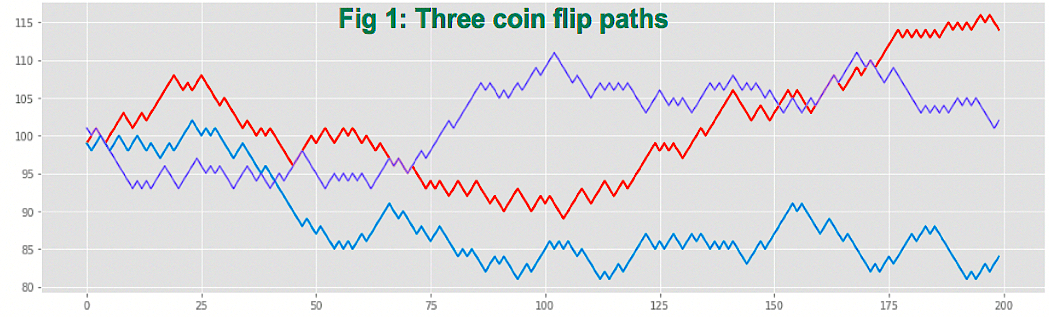
This is ok, as no trade is possible if all market participants have the same viewpoint, but the result of hundreds of thousands of beliefs and viewpoints is that the market is as noisy as a random coin flip, as we observe in Fig. 1, reproducing three paths with 200 coin-flip bets, that closely resembles the paths of a currency or futures market.
 Contradictory strategies may be both profitable or both losers
On my article about trading using bands, profitable trading VII, I’ve described two totally opposed systems: one was a Donchian breakout system, and the other was The Turtle Soup plus one. Both made money and both traded opposite to each other. That shows that opposing beliefs produce profitable systems. Trading is not a competition to decide who’s right and who’s wrong. Trading is a business, and the goal of a trading system is to make money, not being right. In fact, none of these two systems were right even 50% of the time, but both were profitable.
Some time ago I developed a mechanical system and was so wrong that I saw almost a continuous downward equity curve. Nice! I thought. This system is so bad that if I switched it from buy to sell and vice-versa it might result in a great system!
Wrong! The reverse system was almost equally bad. That’s the nature of the markets. Nothing is easy or straightforward.
Too much freedom is dangerous
The marketplace is an open environment where a trader can freely choose entry time, direction, the size of her trade and, finally when to exit. No barrier nor rule forces any constraint on a trader. Such freedom to act is the difference between trading and gambling, but it’s a burden to discretionary traders, especially new to this profession because they tend to fall victim to their biases.
The main biases that a novel trader suffers are two: The need to be right and the belief in the law of small numbers. These two biases combined are the main culprits for the trader’s bias to take profits short and let losses run. The need to be right is also the culprit for the trader’s inclination to prefer high-frequency of winners instead of high-expectancy systems. For more on this read my article Trading, a different perspective.
To counteract this unwanted behavior, we’d need to restrict the trader’s freedom by forcing strict entry and exit rules that guarantee a proper discipline and ensure the expected reward to risk, and, at the same time, avoiding emotionally driven trades.
Discretionary versus systematic
The probability of a discretionary trader to succeed is minimal, mainly because, without a set of rules to enter and to exit, the trader immediately fall into the trap of the law of small numbers and starts doubting his system, usually with a substantial loss, as a consequence of considerable leverage.
Most successful traders develop and improve a trading strategy using discipline and objectivity, but this cannot be qualified as a systematic system because its rules are based on their beliefs about the state of the market, their mental state, and other unquantifiable factors.
A systematic trading approach must, conceptually, include:
- Entry and exit rules should be objective, reproducible, and solely based on their inputs.
- The strategy must be applied with discipline, without emotional bias.
Basically, a systematic strategy is a model of the behavior of one or several markets. This model defines the decision-making process based on the inputs, without emotional or belief content.
Trading can only be successful using a systematic strategy. If a trader does not follow one, trades will not be executed consistently, and there will be the tendency to second-guess signals, take late entries and premature exits.
Personal adaptation
Developing our own trading system not only gives us confidence in its results, but we’d be able to adapt it to our personal preferences and temperament. We don’t like suits that don’t fit well. A system is like a suit. A perfectly good system for one trader might be impossible to trade for another trader. For instance, a trader might not be comfortable trading on strength while another one cannot trade on weakness. A trader may hate the small losses produced by tight stops, so he favors a system with wide stops. That’s why we need to adapt the system to fit us.
The need to measure and keep records
Measurements allow distinguishing good systems from bad ones. There are several parameters worth measuring, that, later, will be dealt with, but the final objective of measurements is to determine if the trading idea behind the system is worthwhile or useless.
Measurements allow finding where the trading system is weak and optimizing the inadequate parameter to a better value. For instance, we might observe that the system experiences sporadic large losses or that it faces too many whipsaws. Measurements allow searching the sweet spot where stops do its duty to protect our capital while preserving most of the profitable trades.
When the system is already trading live, we might use measurements to adapt it to the current conditions of the market, for example to an increase or decrease of volatility. Measurements help us detect when a system no longer performs as designed, by analyzing the current statistical performance against its original or reference.
Discretionary strategies allow measurements, as well, and, sometimes help to improve a particular parameter, as well, particularly stop-loss position, but, how can this help with entries or exits if they are discretionary or emotionally driven?
Measurements, finally, will help us assess proper risk management and position sizing, based on our objectives and the statistical properties of the developed system. This concept will be developed later on, but my previous article Trading, a different perspective, mentioned above, deals with this theme.
Information
In the discretionary trading style the forex information is categorized into the following areas:
- Macroeconomic
- Political
- Asset-class specific
- News driven
- Price and volume
- Order flow or liquidity driven
In the systematic trading style the information is taken from Price and volume, although lately, some systems are also using sentiment analysis, by scanning the social networks (especially Twitter) and news, with machine learning algorithms. Order flow is left to systems designed for institutional trading because retail forex participants don’t have this information.
In this context, systematic trading simplifies information gathering, by focusing mostly on price and its derivatives: averages and technical studies.
Key Features of a sound system
The essential features a system must accomplish are:
Profitability: The model is profitable in a diversified basket of markets and conditions. To guarantee its profitability over time, we should add another feature: Simplicity. Simple rules tend to be more robust than a large pack of rules. With the later, often, we get extremely good back-tested results but this outcome is the result of overfitting, therefore, future results tend to be dismal.
Quality: the model should show a statistical distribution of returns differentiated from a random system. There are several ways to measure this. The Sharpe Ratio and the Sortino Ratio are two of them. Basically, quality measures a ratio between returns and a measure of the variation of those returns, usually this variation is the standard deviation of returns.
Risk Management and position sizing algorithms: Models are executed using position sizing and risk management algorithms, adapted to the objectives and risk tastes of the trader.
It is desirable that the algorithm for entries and exits be separated from risk management and position sizing.
Sharpe Ratio (SR) and other measures of quality
Sharpe Ratio
Sharpe ratio is a measure of the quality of a system, and is the standard way for the computation of risk-adjusted returns.
SR =ER/ STD(R)
SR = Sharpe ratio
R = Annualized percent returns
ER = Excess returns = R – Risk-free rate
STD = Standard deviation
Sortino Ratio
The Sortino Ratio is a variation of the Sharpe Ratio that seeks to measure only the “bad” volatility. Thus, the divisor is STD(R-) where R- is linked solely to the negative returns. That way the index doesn’t punish possible large positive deviations common in trend following strategies.
Sortino Ratio = ER/SRD(R-)
Coefficient of variation(CV)
The coefficient of variation is the ratio of the standard deviation of the expected returns (E), which is the mean of returns, divided by E. It’s a measure of how smooth is the equity curve. The smaller the value, the smoother the equity curve.
CV = STD(E)/E
SQN
The inverse of CV multiplied by the square root of trades is another measure of the quality of the system. It’s a measure of how good it is in comparison with a random system.
SQ = √N x E/STD(E)
Another, very similar measure of quality comes from Van K. Tharp’s SQN:
SQN = 10*E/STD(E), if the number of samples is more than 100 and
SQN = SQ if the number of samples is less than 100.
The capped SQ value allows comparing performance when the number of trades differs between systems.
Calmar Ratio
CR = R% /Max Drawdown%
It typically measures the ratio over a three year period but can be used on any period, and it’s mental peace index. How stressing the system is, compared to its returns.
CR shrinks as position size grows, so it can be a measure of position oversize if it goes below 5
Defining the parts of the problem
To finally produce a good trading system we need to identify, first, the elements of the problem, and at each one of them find the best solutions available. There are many solutions. There’s no question of right or wrong. The optimal solution is the one that fit us best.
1. Identify the tradable markets and its features
The forex market is composed of seven major pairs and 16 crosses. The trader should decide about the composition of his trading basket in a way to minimize the correlation of the currently opened trades.
Liquidity is an important factor too. Especially noteworthy is to detect and avoid the hours when liquidity is low, and define a minimum liquidity to accept a trade.
Volatility is also necessary information that needs to be quantified. Too much volatility on a system designed in less volatile conditions may fail miserably. Especial attention to stop placement if they don’t get automatically adjusted based on the current volatility or price ranges.
We should be careful with news-driven volatility. We must decide if we trade that kind of volatility or not, and, if yes, how to fit that into our system.
2. Identifying the market condition
A trading signal works for a defined market condition. A trend following signal to buy does not work in sideways or down trending markets.
Identify regression to a mean. Usually, mean-reverting conditions happen in short timeframes, due to the spread of trading robots, liquidity availability, and profit taking. Regression to the mean markets merits special entry and exit methods, using some kind of bands or channels, for instance.
Identify oversold and overbought: it is crucial to detect overbought and oversold conditions to avoid trades when it’s too late to get in.
Finally, we must find a way to include all this information in the form of a set-up or trading filter.
3. The concept and yourself
There are lots of ways to trade a market, but not every one of them will fit all traders. An example of a tough system for myself would be the Donchian breakout system. A robust and simple trend following system, but I know I wouldn’t be comfortable with 35% winners because I know that this means 12% chance of having a streak of 5 losers.
Therefore, to know what fits you, you should try to know yourself and your available time for trading.
Conceptually there are two kinds of players: Those who need frequent small gains and accepts sporadic substantial losses (premium sellers) and those who are willing to pay insurance for disasters, taking periodic small losses in search of large gains (premium buyers).
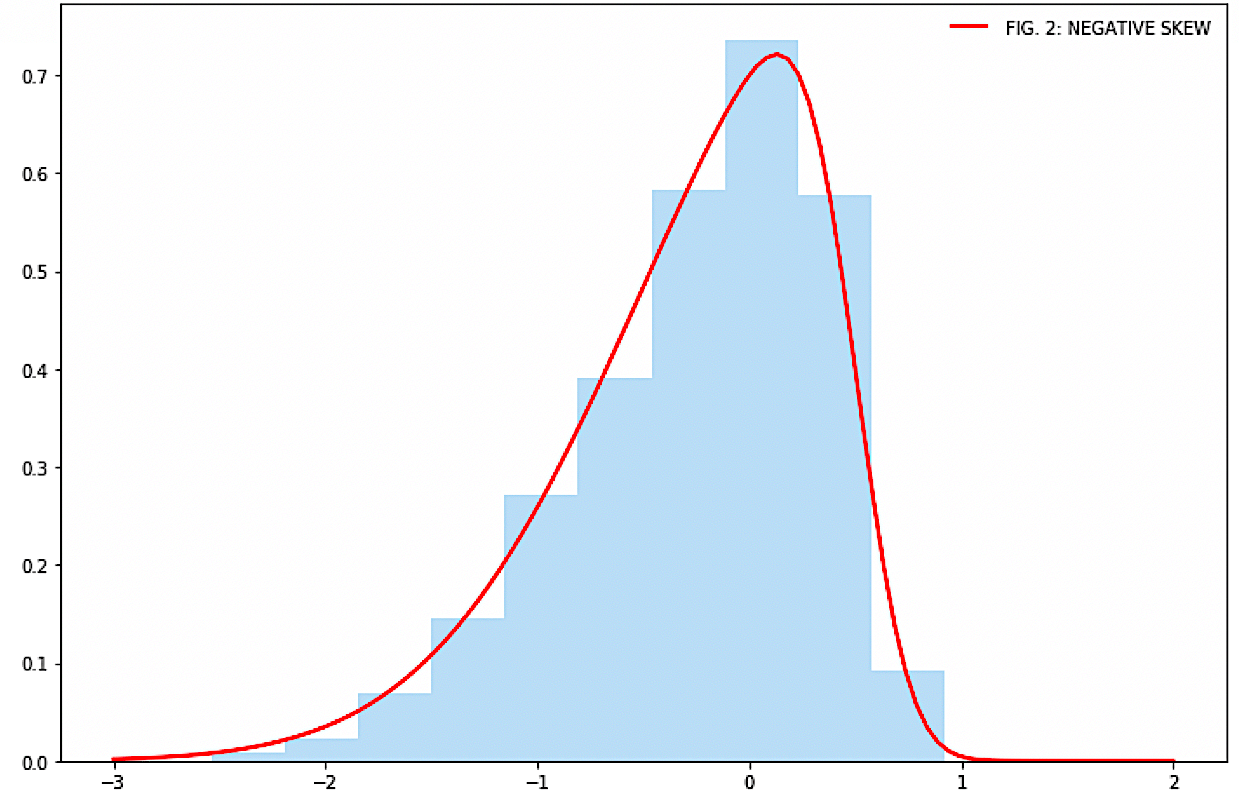
A premium seeker prefers a hit-and-run style of trading: scalping, mean-reverting, swing trading, support- resistance plays, and similar strategies. A premium seeker has a negatively skewed return distribution, as in Fig. 2:

A premium buyer is a trend follower, an early loss taker, a lottery ticket buyer, a scientist experimenting in search of the cancer cure. He is willing to be wrong several times in a row, looking for the big success: W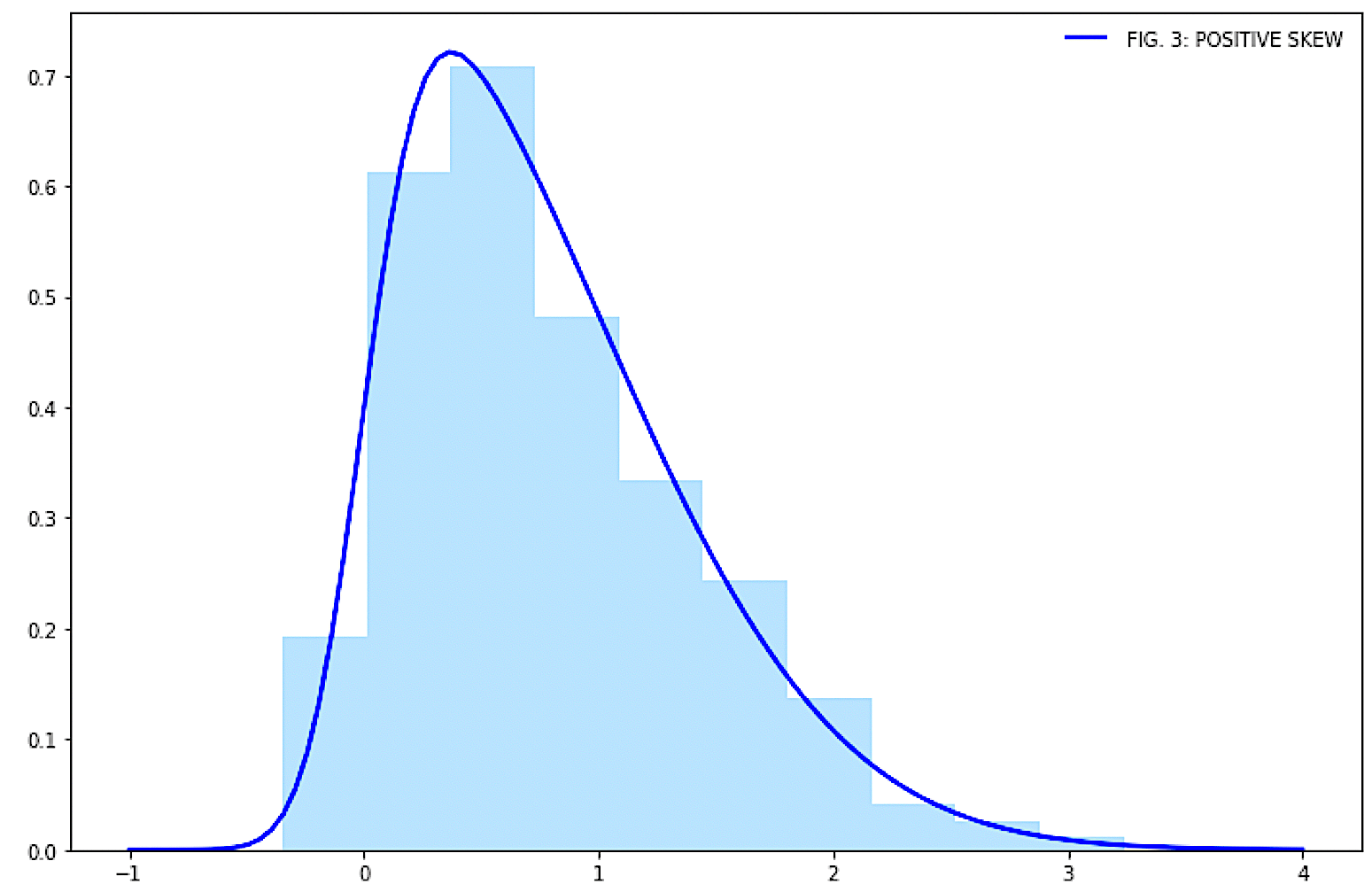 hen he finds a trend, he jumps on it with no stops. If proven right, he adds to the position, pyramiding, as soon as new profits allow it. A premium buyer has a positively skewed return distribution, as in Fig. 3:

We notice that the most psychologically pleasing style comes from premium-sellers. The problem with this trading style is that it is not insured for the black-swan-type of risks. He is the risk insurer!
The premium buyer is like a businessperson. A person who is willing to assume the cost of the business for a proper reward. His problem is that he must endure continuous streaks of small loses.
An early loss taker is against the crowd instinct to take profits early, a habit with a negative expectancy, so it pays extra returns to be contrarian.
There is a mixed style where reward to risk is analyzed and optimized. It uses stop protection, while the percentage of winners is enhanced using profit targets.
The main concept for a sound system, in my opinion, is to make sure our distribution of returns has a positive skew. That can be accomplished if we make sure our system has a mean reward-to-risk ratio higher than 1:1, preferably greater than 2:1 but never less than 1:1, and by setting profit targets in tune with the market movements – placing them near resistance or support, and using trail stops.
4. The law of active management
The Fundamental Law of Active Management was developed by Grinold and Kahn to measure the value of active management, expressed by the information ratio, using only two variables: Manager skill IC and the number of independent investment opportunities N.
IR = IC x √N
If two managers have the same investment skills but one has a more dynamic management, meaning N is higher than the other manager, its return will outperform the less dynamic manager.
This formula can be used in trading strategies, as well: On two equally smart strategies, the one with more frequent trading will outperform the other. There’s a limitation, though, that this formula doesn’t address: The cost of doing business is more significant the higher the frequency of trading.
5. Timeframes: Fast vs Slow
The trader’s available daily time has to be considered too. Does the trader have time to be on the screen the whole day or are they busy during work hours, hence, only able to dedicate just a couple of hours at noon to trading.
Unless the trader is willing to use a fully automated system, the time available to them dictates the possible timeframes. A trader who’s busy all day cannot trade signals that show on 1-hour timeframes but is instead forced to focus on swing trading signals that can be analyzed at noon. A full-time trader has all available time-frames at their disposal.
Well summarize here the classification made by Robert Carver on his book Systematic Trading:
· Very Slow (average holding period: months)
Very slow systems tend to behave like buy and hold portfolios. Trading rules tend to include mean reversion to very long equilibrium such as relative value equity portfolios, that buy on weakness and sell on strength.
As a result of the law of active management, returns from dynamic trading diminish, the lower the trading frequency. Therefore, at large holding periods, the return tends to be poor, unless the skill at timing the market were top notch.
· Medium (average period hours to days)
The law of active management gives us a clue that this timeframe gets more attractive results than a longer time-frame.
It’s adequate to part-time traders that can do swing trading, working in the evening, searching for signals to be used in hourly and daily charts. From a Forex perspective, these medium-speed timeframes are less crowded with traders. Therefore, strategies may work better than shorter timeframes.
· Fast( from microseconds to one day)
The Sharpe ratios could be very high in these timeframes, an important portion of the raw returns ought to be spent on costs (commissions and spreads).
6. Risk
Risk is a broad concept. There are several kinds of risk. The first type of risk is the trade risk. The risk you assume on a particular trade. That’s the monetary distance from entry to your stop loss multiplied by the number of contracts bought or sold. It’s easy to assess and measure.
The second type of risk is the Potential drawdown a system may experience. This kind of risk is dependent on position size and the percent losers of the system, therefore, we can estimate it with certain accuracy.
Risk can be defined as the variability of results. It’s a statistical value that measures the mean value of the distance between results, and the mean of results and is called standard deviation. The point is that market volatility is shifting and, further, it’s different from asset to asset.
If a trader has a basket of tradable markets, there might happen that one asset is responsible for 60% of the overall volatility on her portfolio, because the position size in that particular asset is higher, compared with others or because its volatility is much higher.
The best way to reduce the overall risk is through diversification and volatility standardization.
Diversification:
To reduce overall risk, there is just one solution: To trade a basket of uncorrelated markets and systems, with risk-adjusted position sizing, so no single market holds a significant portion of the total risk.
Below is the equation of the risk of an n-asset portfolio when there’s no correlation:
𝜎 =√ ( w1 𝜎12 + w2 𝜎22 + … + wn 𝜎n2)
where 𝜎I is the risk on an asset, and wi is the weight of that asset on the basket.
Let’s assume that we hold a basket of equal risk-adjusted positions in 5 uncorrelated markets with a total risk of $10. Therefore, we have a $2 risk exposure on each market, and the correlated total risk would have been 10. But, if the assets were totally uncorrelated, the expected combined risk would be computed using the above equation, then:
Risk =√ (5 x 22) = √20 = 4.47
So, for the same total market exposure, we have lowered our risk by more than half.
Volatility standardisation
Volatility standardization is a powerful idea: It is the adjustment of the position size of different assets, so they have the same expected risk.
This allows having a balanced portfolio where each component has a similar risk. It means, also, that the same trading rule can be applied to different markets if applied with the same standardized risk.
Leverage
The forex industry is attractive for its huge amount of allowed leverage. A trader is allowed to control up to one million euros with a modest 10,000 euro account. That is heaven and hell at the same time. If a trader doesn’t know how to control her risk, he’s surely overtrading.
I recommend reading my small article on position size, but for the sake of clarity, let’s do an exercise.
Let’s compute the maximum dollar risk on a $10,000 account and a maximum tolerable drawdown of 20%, assuming we wanted to withstand 8 consecutive losses.
According to this, we will assume a streak of eight consecutive losses, or 8R.
20% x $10,000 = $2,000 this is our maximum allowed drawdown, and will be distributed over 8 trades, so:
8R = $2,000 = $250, therefore:
Our maximum allowed risk on any trade would be $250 or 2.5% of our running account.
By the way, that value is a bit high. I’d recommend new traders starting with no more than 0.5% risk while beginning with a new system. It’s better to pay less while learning.
The second part of the equation is to compute how many contracts to buy on a particular entry signal.
The risk on one unit is a direct calculation of the difference in points, ticks, pips or cents from entry point to the stop loss multiplied by the minimum allowed lot.
Consider, for example, the risk of a micro-lot of the EUR/USD pair in the following short entry:
Size of a micro-lot: 1,000 units
Entry point: 1.19344
Stop loss: 1.19621
We see that the distance from entry to stop loss is 0.00277
Then, the monetary risk for one micro-lot: 0.00277 * 1,000 = € 2.77
Therefore, the proper position size is €250 /€2.77= 90 micro-lots, or 9 mini-lots
Using this concept, we can standardize our position size according to individual risk. For instance, if the unit risk in the previous example were $5 instead, the position size would be:
PS = €250/5 => 50 micro-lots.
That way risk is constant and independent of the distance from entry to stop.
Finally, it’s better to use a percentage of the running capital instead of a fixed euro amount, because, that way, our risk is constantly adapted to our current portfolio size.
7. The profitability rule
A trading system is profitable over a period if the amount won is higher than the amount lost:
∑Won -∑Lost >0 (1)
The average winning trade is the sum won divided by the number of winning traders Nw.
W =∑Won / Nw (2)
The average losing trade is then:
L =∑Lost / NL, (3) where NL is the number of losing trades.
Thus, equation (1) becomes:
WNw – LNL, > 0 (4)
The number of losing trades is the total number of trades minus the winning trades:
NL = N – Nw (5)
Therefore, substituting (5) and dividing by N, equation (4) becomes:
WNw / N – L(N-Nw) / N > 0 (6)
If we define P = Nw / N, then (N-Nw) / N = 1-P, and (6) becomes:
WP– L(1-P) > 0 -> W/L x P – (1-P) > 0 (7)
Finally, if we define a Reward to risk ratio as Rwr = W/L Then we get
P > 1 / (1+ Rwr) (8)
Equation 8 is the formula that tells the trader the minimum percent winners required on a system to be profitable if its mean reward to risk ratio is Rwr.
Of course, we could solve the problem of the minimum Rwr required on a system with percent winners greater than P.
Rwr > (1-P)/P (9)
8. Parts of a trading system
In upcoming articles, we’ll be discussing all parts of a trading system extensively. Here we are just sketching a skeleton on which to build a successful system.
A trading system is composed of at least of a rule to enter the market and a rule to exit, but it may include the following:
- A setup rule: A rule defines under which conditions a trade is allowed, for example, a trend following rule.
- A filter rule: A filter to forbid entries under certain conditions, for example, when there is low volume, or high volatility, the overbought or oversold conditions are reached.
- An entry rule, defined with price action, moving averages, MACD, Bollinger Bands and so on.
- A stop-loss, to limit losses in case the trade goes wrong. Optionally a trailing stop.
- A profit target: Profit target may be monetary, percent, based on supports or resistances, on the touch of a moving average or any other.
- A position sizing rule. As mentioned before, it should make sure the risk is evenly and correctly set.
- Optionally, A re-entry rule. The rule decides a re-entry if the stopped trade turns again on the original trade direction.
9. Chart flow of the development of a trading system


In the next chapters of this series, we will develop on every aspect sketched in this introductory article.
References:
Professional Automated Trading, Eugene A. Durenard
Systematic Trading, Robert Carver
Profitability and Systematic Trading, Michael Harris
Computer Analysis of the Futures Markets, Charles LeBeau, George Lucas
Building Winning Algorithmic Trading Systems, Kevin J. Davey


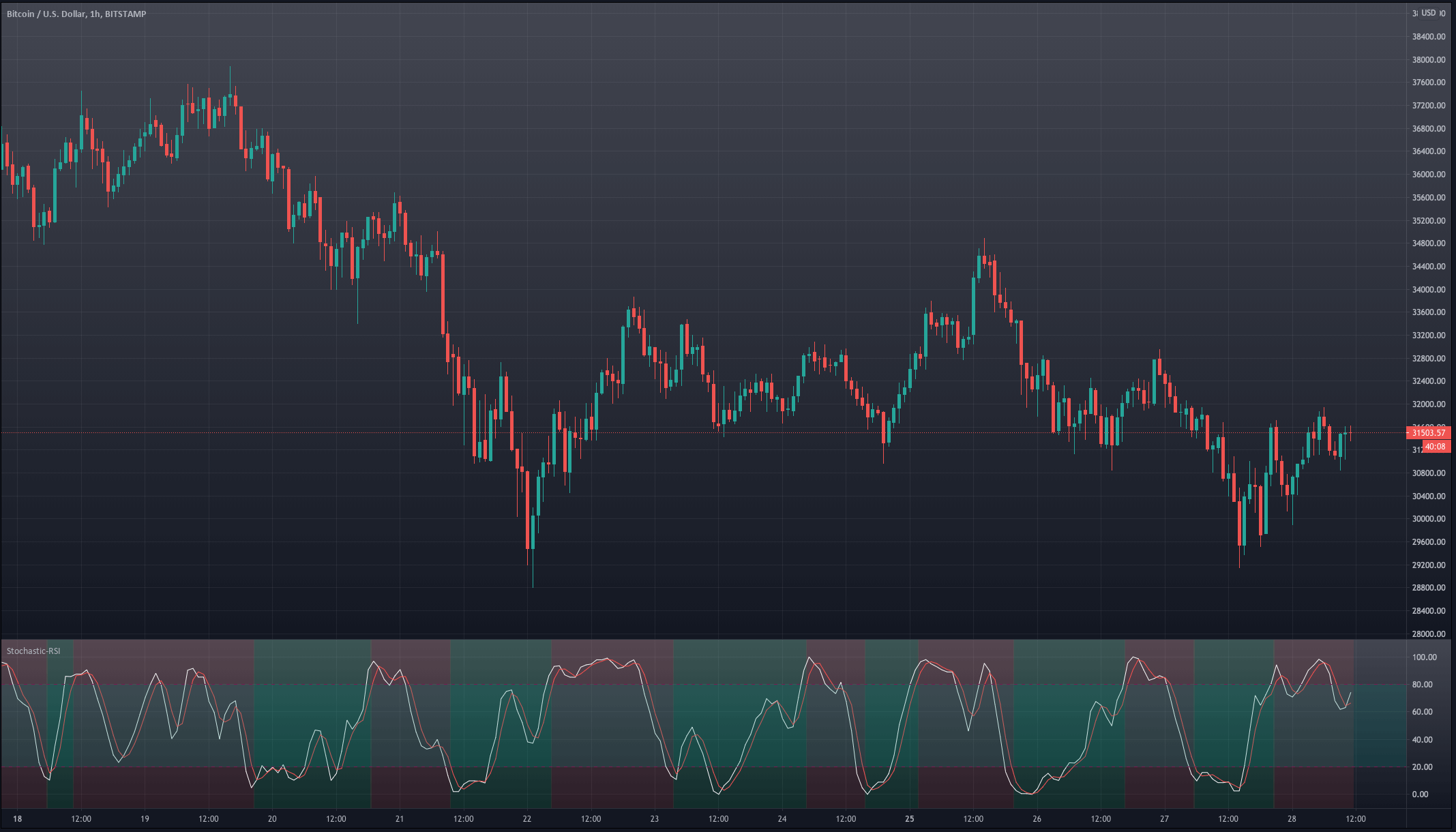 Variant 1 triggers the transitions too early. We see that on many occasions when the stochastic RSI enters the overbought or oversold region, it is more a signal of trend strength than a turning point.
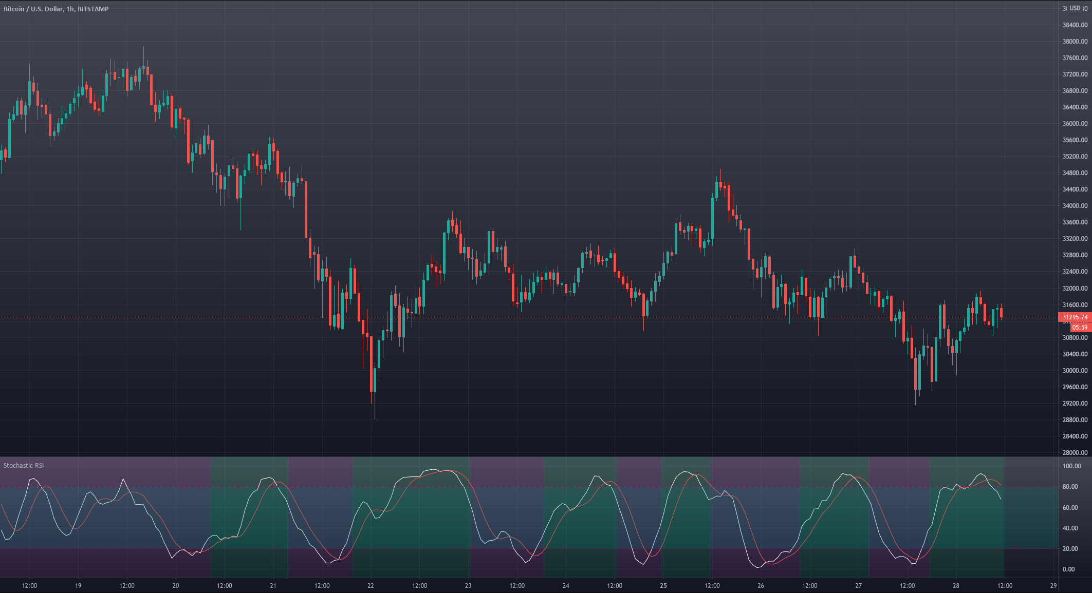
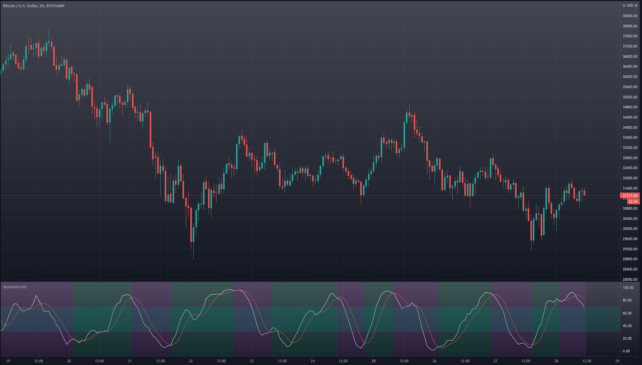


 Forex traders usually get MT4 for free when opening a trading account, and MT4 includes what it calls a “strategy tester” which is accessible by clicking a magnifying glass button or Ctrl-R.