Categories
Forex Basic Strategies

Understanding Welles Wilder PSAR Indicator

Introduction

The Parabolic Stop and Reverse system was presented by Welles Wilder in his classic book New Concepts in Technical Trading in 1978, and he originally calls it The Parabolic Time/Price System.

This system sets stops at points that are closer and closer to the price action as time goes on. Mr. Wilder calls it “parabolic” by the fact that the pattern forms a kind of parabola when charted. The main idea is to give the market room at the beginning of the trade and, as price moves in our favor, gradually tighten the stops as a function of time and price.

The PSAR stop always moves in the direction of the trade, as a trailing stop should do, but the amount it moves is a function of price because the distance the stop level is computed relative to the range the price has moved. It also gets closer to the price action regardless of the direction of the price movement.

PSAR equation

If the stop is hit, the system reverses; therefore, Wilder named each point SAR: Stop and Reverse point.

The formula to compute it is:

 SARTomorrow = SARToday + AF x (EPTrade – SARToday)

The AF parameter starts at 0.02 and is increased by 0.02 each bar with a new high until a value of 0.2 is reached.

The EP  parameter is the Extreme Price point for the trade made. If long, EP is the highest value reached. If short, EP is the lowest value for the trade.

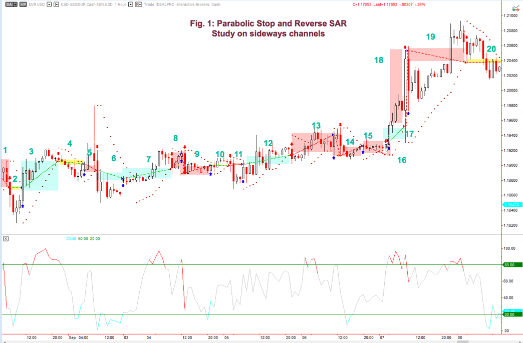
Fig 1: The magenta areas are winners, the yellow are break-even trades, and the pink regions are losers. As we might expect, in congestion areas, the SAR system is a loser.

The PSAR Trading System

PSAR as a naked system isn’t too good, since trades that go against the primary trend tends to fail, and almost all trades fail when the price is not trending. Sudden volatility peaks also fool the PSAR system. See Fig 1, point 18, where an unexpected downward peak reversed the trade in the wrong direction, cutting short a nice trade and transforming it into a big loser.

Fig 2a and 2b show the profit curve for longs and shorts in the EUR/USD 1H EURUSD 2017 chart. As expected, the long-trade graph presents more robustness than the short-trade curve, since the EURUSD had a clear upward trend back in 2017, whereas the short trades lost money. That is an example of how following the underlying trend grant traders an edge.

Fig 2a equity curve for long trades

Fig. 2b – Equity curve for short trades

Anyway, it’s fantastic that using an entry system with absolutely no optimization could deliver such good results as the  PSAR system when taking only the trades that go with the primary trend. That shows, also, the power of a good trailing stop.

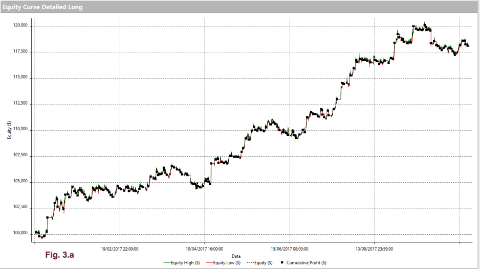
The naked system isn’t too good at optimizing profits, as well. A profit target makes it a lot better. Fig 3.a and Fig. 3.b shows the improvement after setting an optimal target for longs and shorts, especially relevant on shorts.

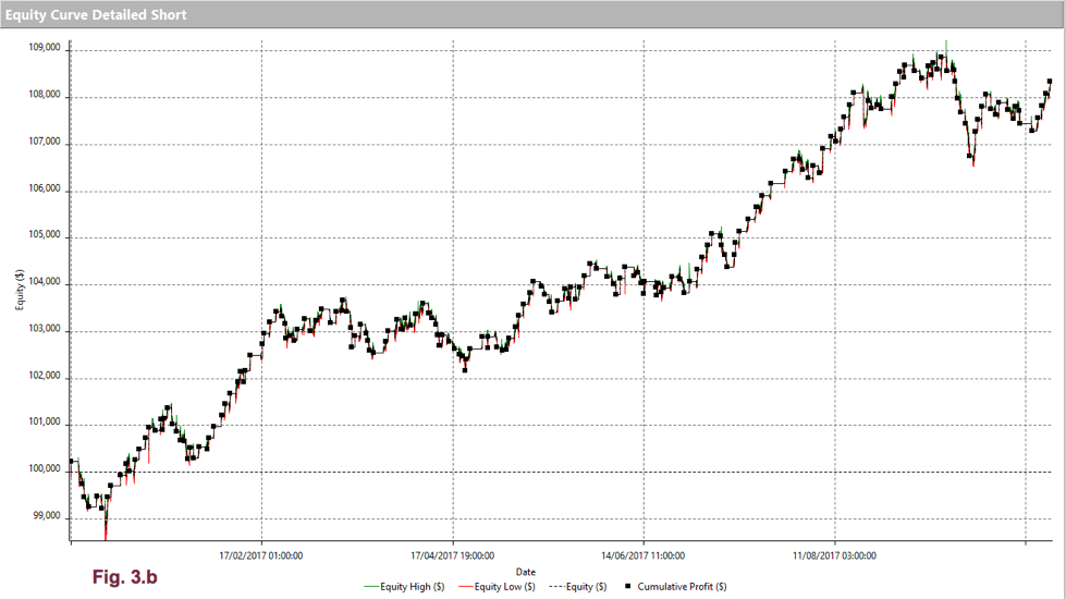
A small change in the AF parameter, lowering down to 0.18, to give profits more room run, and the use of profit targets, raised the percent profitable from 41.4% to 48.1. Max drawdown improved from -4.77% to -3.37%, as well, and the avg_win/avg_loss ratio went from 1.69 to 1.78. It seems not too much, but in combination with the increment in percent winners to 48.1% makes it an effective and robust system.

PSAR as a trailing stop

In this section, we’ll study the Parabolic Stop and (not) Reverse system, as it might be called, as the exit part of a trading system.

As an exercise, let’s consider a simple moving average crossover. We’ll use the same market segment that we used in the naked PSAR case. For longs, we’ll use an 8-15 SMA crossover, while, for shorts, a 7-23 SMA will be taken, as this arrangement creates optimal crossovers for the current market.

Figs. 4a and 4.b show the equity curve for longs and shorts, respectively, with a Simple Moving Average Crossover system, acting on its own. No PSAR stops added.

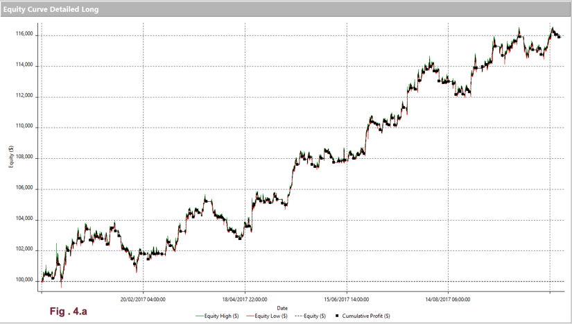
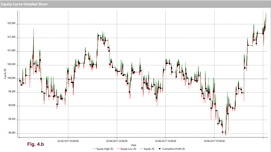
As we see in fig 4a, the long equity curve behaved much better than the short one, although that is due to the EUR/USD trending up. On the short side, even after optimizing its parameters, the crossover relationship is lousy.

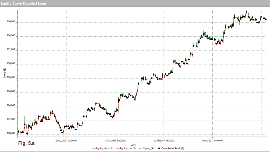
Fig 5.a and 5.b show the effect of a PSAR trail stop. There’s almost no noticeable positive effect. The oddity that PSAR, as a system, is more profitable than when it acts as a trailing stop in another system is related to the entry signal. It’s evident that the SAR signal takes place earlier than the SMA crossover, so the PSAR stop isn’t able to extract profits when the entry signal lags its own signal. On the short side, if we take a closer look, we can see that it improves a bit the drawdown.

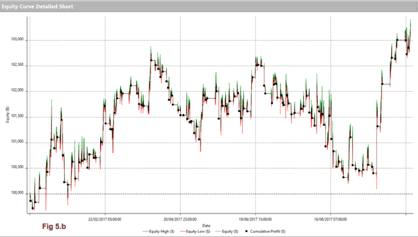
It may seem that the smart thing to do in a trending market such as the EUR/USD back in 2017 is NOT to trade the short side, at least not mechanically.

Take-Profit Targets

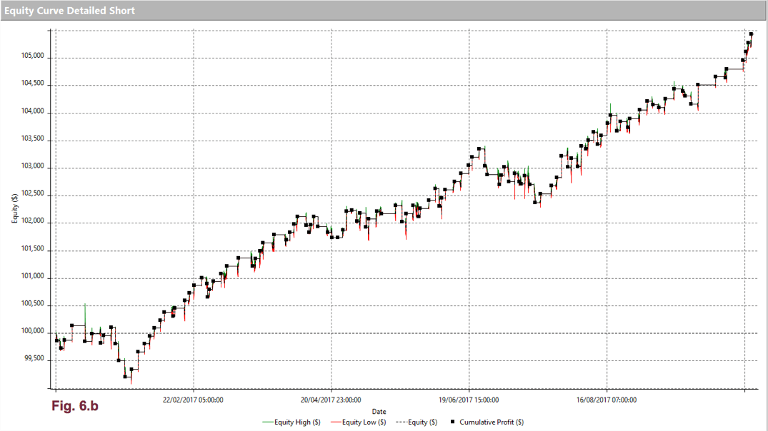
But, it’s impressive how take-profit targets help us extract profits and reduce risk when trading against the trend. Let’s see the equity curves using long and short targets:

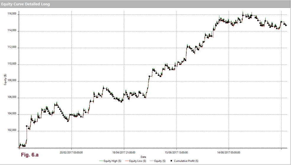
We observe that the long equity curve has a bit less drawdown, but, overall, it doesn’t change much. That was expected because the naked crossovers are very good at following a trend, so not very much can be gained using targets.

The use of profit targets is much more noticeable on the short side. It not only presents a higher final profit, but it’s drawdown practically disappeared, allowing us to better extract profits against the prevailing trend. We have to be cautious, though, if we detect a major trend change and adapt the targets accordingly.

Conclusions

Throughout this article, we tried to understand and analyze the PSAR as, both, an entry-exit system and its behavior as trailing stop to be used with other entry systems. We spotted its strengths and its weaknesses.

Given the results of our present study, we can conclude that:

  • The PSAR is a decent system if we combine it with a market filter and profit targets.
  • Trailing stops, even sophisticated ones, such as PSAR, doesn’t solve our problem of whipsaws when we trade against the trend.
  • By tweaking a bit the AF parameter down to .18, we were able to improve the trend following the nature of PSAR. Consequently, it is advisable to adapt PSAR to the current market volatility.
  • The best tool we own to profit using counter-trend strategies is profit targets, optimized to the current swing levels of the market.


References:

The definition of the PSAR is taken from New Concepts in technical trading, Welles Wilder.

The studies presented were made using Multicharts 11 trading platform programming capabilities, and its results and graphs were taken from its System Performance Report.

Categories
Forex Educational Library

Profitable Trading – Computerised Studies I: DMI and ADX

Introduction

The spread of personal computers gave investors and traders the opportunity to perform sophisticated computations in an attempt to extract information out of the naked price series. Many traders believe there’s a hidden structure in the markets, and the harder and computationally difficult the indicator is (such as ARIMA, MESA or Fourier analysis) the better. Unfortunately, until now, no computational formula reveals the secret turns of the markets, and if there is one, I don’t think the person or organisation that owns it will show it to the rest of us. But I honestly believe there’s no such formula. The era of deterministic theories of reality is gone. That is clear to me since I’ve been introduced to the quantum theory of physics. More on this: http://www.hawking.org.uk/godel-and-the-end-of-physics.html

But that doesn’t mean technical studies are worthless. There are well known and relatively simple indicators designed to give us information difficult to see or detect by just looking at the price movement, or at least to help us confirm the pattern that price is shaping.

In this article, we’ll study Welles Wilder’s DMI/ADX study

Directional Movement Index (DMI) and Average Directional Movement Index (ADX):

This study came to answer two questions by trend followers: Is there a trend or not? And how strong is it? And these issues aren’t trivial. Trend following traders looks to enter as soon as possible on a trend, usually on breakouts. But, if the market isn’t trending, they enter on a breakout and watch their initial profit become a loss as the breakout fails.

The proper interpretation of ADX help traders to avoid potential losses due to false breakouts, helping them focus on trendy markets, and apply other trading tactics when the signal shows the market isn’t trending.

DMI concept

Directional Movement was developed by J. Welles Wilder Jr, and described in his book New Concepts in Technical Trading System (1968). The DMI indicator is a very useful technical study that shows the market direction. One DMI derivation, the ADX, allows us to quantify the strength of a trend.

The directional movement DI is based on the idea that if the trend is up, the current bar’s high should be above the previous bar high. Conversely, if the trend is down then the current bar’s low should be lower than on the former bar. The difference between the current high and the previous one yields +DI, while, the difference between the current low and the previous one results in –DI. Inside bars are ignored.

  1. If the current bar’s range moves above the previous bar’s range, there’s a new +DM value; while –DI = 0
  2. If the current bar’s range goes below the previous bar range, there’s a new –DM value, while +DI = 0
  3. Outside bars (whose low and high are beyond yesterday’s range) will have both, positive and negative DM. The larger will be used and the shorter equated to zero.
  4. On an outside bar, if both values are equal, then both DM =0
  5. On Inside bars, both DM = 0

Computation of the DMI

DI, the directional indicator, is computed by dividing DM by the True Range (TR).

DI = DM / TR

TR, the true range is the biggest of these three quantities:

High – low

High – close

Close-low

The resulting DI calculation may be positive or negative. If positive (+DI), it’s the percentage of the current bar’s true range that’s up. If negative (-DI), it’s the percentage that’s down for that bar.

The DI’s are averaged over a period. Mr. Wilder suggests 14 bars.

The calculation for 14 bars is:

+DI14 = DM14 / TR14

Where DM14 and TR14 are the averages of those quantities over a 14 bar period.

ADX is derived from +DI and +DI, using the following steps:

  1. The absolute difference is computed:

DIdiff = | [(+DI) – (-DI)] |

  1. The sum is, also, computed:

DIsum = [(+DI) + (-DI)]

  1. Compute DX:

DX = 100 x DIdiff / DIsum

The 100 scales the DX values between 0 and 100.

DX is too wild to be used directly, so we compute a moving average of DX and call it Average Directional Indicator, ADX. Usually, the smoothing average has the same period as the one used to obtain the DI.

Another indicator may be created using a momentum-like derivation of ADX called Average Directional Movement Index Rating (ADXR)

ADXR = (ADX – ADXn) / 2

Where ADX is the value for the current bar and ADXn is the ADX for the nth bar ago.

When drawn on a chart, if +DI is above –DI, then the trend is up. The opposite situation means a downward move.

If the two lines diverge, the directional movement increases. The greater the difference, the stronger the trend.

According to Wilder, the 14-period averaging was chosen because of his idea of a half cycle. Day or swing traders may choose to modify it based on the half cycle of the time frame he is trading. For instance, LeBeau and Lucas in their book recommend 12 bar averaging on a 5-min chart.

Fig 2 shows the hourly EUR/USD and the DMI & ADX study. We observe that on the left quarter, when there’s no trend, the ADX is below 25, touching the +DI and -DI lines; and these lines themselves are crossing over each other every few bars. Then a breakout in price matches the growth of the ADX line, while +DI crosses over –DI. The ADX signal grows while the trend keeps moving up with increasing strength.

The top formation changes its character and goes down following the price until –DI crosses over +DI and, then, ADX starts growing again, while price keeps falling: A downtrend is confirmed.

The sideways channel forming a local bottom hurts the ADX again, and then the small reaction up (+DI crosses over -DI) moves it up. Then the sudden drop in 5 bars makes a slight dip but ADX is up again.  Then, on a new price floor (support), ADX drops again, and so on.

It seems sluggish and untimely. Many people discard it because of that. But we must remember the ADX indicator shows only trend strength.

The DI system tracks the fight between bulls and bears. It measures the power of bulls and bears to move prices beyond the previous bar range. When +DI is above -DI it shows that bullish sentiment has dominated the market so far. -DI above +DI shows the bears are in control. Thus, following the direction of the upper line is an edge.

ADX rises when the spread between +DI and –DI grows. It shows that the market sentiment (bull or bear) of the dominant market group gains strength, so the trend is probably continuing.

ADX drops when +DI and –DI are approaching each other. This shows that the dominant group is losing strength and the health of the trend is in question.

Rules for trading with ADX and ± DI:

The real value is as a filter for entries.  It’s important to understand that the ADX alone doesn’t show market direction, but the strength of a trend. We should use the +DI and -DI crossovers to determine direction.

  • If +DI is above –DI then the trend is up. If the opposite is true, there’s a downtrend. Consequently, we filter trades opposite to the current trend direction.
  • When the ADX declines, it’s an indication of a market top, and we should exit the trade or tighten stops. While ADX is pointing down, it’s better not to use any entry methods designed for trend following.
  • When the ADX is below or touching the DI lines, it signals a sideways channel or flat market. Under these conditions, breakouts have higher probabilities to fail. We should wait for ADX to go up again.
  • The ADX line below both lines is a sign of very low volatility, and, for sure, we are in a very quiet sideways channel. Therefore, it’s an excellent opportunity to take the breakout of the channel, since the reward to risk should be attractive.
  • When the ADX is well above the two lines, it may signal an overbought or oversold market condition. When the ADX stalls it may be time to take profits, reducing positions or tightening stops.

References:

Computer Analysis of the Futures Markets, Charles LeBeau and David W. Lucas.

The New Trading for a Living, Alexander Elder.


Categories
Forex Educational Library

Profitable Trading VIII – Computerized Studies V: Oscillators

Introduction

Markets behave as a fair-price searching machine. When there is no consensus about value, caused by an economic event or some other news that might affect the current fair price, market forces launch a new trend, which starts moving the price toward another “fair” level.

And the rest of the time, when the price is already at a consensus “fair price”, what happens? Does it stay at a single price point until a new event shakes it?

Nature hates stillness and rest. It seeks movement -Any kind of movement- and the markets do, as well. Therefore, as we all acknowledge, price does not stay still just because everybody on earth thinks this is the fair price. The fact that there are zillions of market participants, every one of them with its own opinions, makes it impossible that a fair price exists at all. As Jesse Livermore stated, the two most significant market forces are greed and fear, and, consequently, they exert their pressure on prices, too.

Therefore, when a market lacks impulse to continue a trend, it tends to make oscillatory price changes, although the fact that traders are using different time frames, price targets, and stops, makes this oscillation quite complex, with multiple cycles blended on an intricate and, potentially, noisy pattern.

Science has been dealing with waves and cycles for long. Almost everything in science deals with cycles and oscillations, therefore, cycles are a part of markets that may be handled with precise scientific accuracy, limited only by the noisy nature of prices.

To conclude, Markets mainly behave in two interlinked modes: trend mode and cyclic mode. Those two states may blend with each other on a higher timeframe, though.

We’ve already dealt with computerized studies to help traders find and trade a trend. In this article, we’re going to analyze several computerized studies which might assist us during the cyclic phase of the market, when the markets are not trending.

Slow Stochastics

The Stochastics oscillator was developed by George Lane, who teach it during his investment seminars since 1950. According to Lucas and LeBeau on his book “Computer Analysis of the Futures Markets”, Mr. Lane has been perfecting the use of stochastics for trading over many years, and he is able to make it work well in almost any market situation.

The Stochastics Oscillator, came from the observation that closing prices tend to appear near the high of the range during uptrends and near the low of the range in downtrends.

This oscillator measures where the close is, relative to the range of prices over the latest period. The %K line comes from a simple formula, which makes sure the signal is always between zero and 100:

There is a %D line, which is called slow stochastic and is computed by applying a three-day moving average to the %K line.

By convention, an overbought market is one that led its stochastics lines – %K and %D – above the +80 level; while a market is in oversold condition when they are below the 20 level.

The basic way to use Stochastics is by acting at %D and %K crossovers when this happens at those extremes, and when the %D line crosses – over or under- these price triggers. For example, when %D crosses under the 80 level it indicates a sell signal, and when it crosses over the 20 level, it’s a buy signal.

Periods

The standard period for the Stochastic oscillator is 14, but, according to Lucas and LeBeau, George Lane used an adjusted value of about 50% of the perceived market main cycle. Those authors said in their book that they had tested several periods, and a range between 9 and 12 were the best performing ones, as these were the best compromise between speed and validity, producing the minimum quantity of false signals.

What this tells us is that we need to experiment with the period of the signal and back-test it, to get an optimal figure for the current market we are treading.

According to Alexander Elder, if you intend to use Stochastics as your sole signal it’s better to choose a longer-term period, while in combination with other signals a shorter period is preferable.

Signals against the trend

As said at the beginning, the use of this kind of oscillator is best suited to a cyclic phase of the market. When we detect a trend, the Stochastic oscillator does not perform so well, especially when the signal is against the main trend.

Fig. 2 shows a stochastics used in a downtrending market (NZD/YSD). We may observe that, mostly, good signals come from the overbought side of the market that trigger signals with the trend, even when those appear before %K and %D approaches the saturated region. This is common with strong trends. The market doesn’t reach the overbought ( or oversold) level before returning to the primary trend. The only potentially profitable buy signal comes at the end of this long downtrend when the oversold condition permeates several time frames.

LeBeau and Lucas said in his book: “Remember: The trader who coined the phrase ‘the trend is your friend’ was not using stochastics”.

Divergences

Several authors agree about the fact that divergence between prices and stochastics is one of the most powerful signals.

A bullish divergence occurs when a price makes a new low and the stochastic fails to do so, drawing a higher low.

A bearish divergence arises then prices are making new highs but stochastics lines draw a lower low.

A word of caution about divergences: It may work or not. I don’t know for sure. What’s sure is its performance is very challenging to test. I’d rather like those signals that I’m able to back-test, such crossovers, departures from an overbought or oversold level,  etc.

Knees and Shoulders

When %K has crossed over %D and, then, pulls back, but, without another %D crossing to the downside, and, next, it resumes its up movement, Mr. Lane calls it a knee. If the movement is from overbought to the downside, he calls it a shoulder. According to Mr. Lane, it shows a continuation with strength.

Anticipating a crossover

There are people that remark when %D flattens, call it a hinge. Also, there’s a warning hook, when both %K and %D turns at an extreme but still don’t cross.

According to LeBeau and Lucas, those observations focus, mainly, on anticipation rather than reliance on the signals, and they don’t recommend them. It’s better to wait for a crossover.

Bear and bull setups

Another unique tool by George Lane.

A bear setup happens when prices make a series of higher highs and higher bottoms, but the Stochastics oscillator produces a pattern of lower lows when prices are rising. This pattern indicates there will be a top soon.

Bull setups are the specular pattern to bear setups, indicating that a bottom will happen soon.

Williams %R

Williams Percent R is a momentum indicator developed by Larry Williams, very similar to the Stochastic indicator, but in this case, it computes the level of the closing price in relation to the highest high of the period, instead of the lowest low, and it doesn’t depict a smoothed %D line.


Therefore, this oscillator moves from -100 to 0. Values below -80 are oversold levels while from -20 to 0 are overbought levels.

Some charting packages shift these values to positive 0 to 100 by adding 100 to the formula. In this case, oversold levels are between 0 and 20, and overbought condition happens from 80 to 100.

%R is noisier than Stochastic %D, but with less lag, so together with a confirming pattern,  it usually allows for a better reward to risk ratio and tends to show more trade opportunities than Stochastic does.


This indicator is very good at detecting oversold conditions at an uptrend, or overbought levels at a downtrend, therefore, it’s well suited as a signal, to add to a position or enter a new one on pullbacks.


Advanced topics:

Adaptive Stochastics Indicator

John Ehlers introduced the idea of an adaptive indicator in his book “Cycle Analytics for traders.” Ehlers proposes to, first, find the dominant cycle first, and then use half of that cycle as the period for the stochastic calculation.

So, the adaptive Stochastics starts by computing the dominant cycle using an autocorrelation periodogram, which Ehlers describes in chapter 8 of his book (I will refer the interested readers to check it).

In his book, Ehlers showed the complete algorithm, as well (although written in easy-language, it may be transposed to any language). The main steps are:

  • A low pass roofing filter to eliminate unwanted noise from the price data
  • The periodogram calculation
  • The instantaneous period is used to compute the current value of %D.
  • No %K is computed.

As we observe from fig. 8, the adaptive stochastic is much less noisy and it adapts to the dominant cycle.

Center Of Gravity

John Ehlers describes this oscillator in chapter 5 of his book “Cybernetic analysis for stocks and futures, cutting edge DSP technology to improve your trading”. He states that this study is unique because his smoothing has virtually zero lag, therefore, enabling a definite identification of turning points at the same time.

The center of gravity of an object is, basically, a weighted center of its mass, a balance point. In a trading environment, we can define a kind of rule of weights on an observation window. A fast and upward moving price shifts the center of prices to the right, while a downward move, shift it to the left.

The following formula computes CG:

CG = ∑i=0 to N (xi +1) * Pricei / ∑ i = 0 to N   Pricei

Fig 9 shows the EUR/USD 10-minute chart with Center of Gravity. As we clearly see, the CG is almost free of noise, so a signal can be picked directly from its crossovers if they happen relatively far from its zero line.

Cyan and pink boxes on Fig.9 show the result of scalping on a 10-min EUR/USD chart using CG crossovers. Nothing is perfect in trading, but we clearly observe that CG crossover signals catch the turning points with accuracy, allowing a highly probabilistic approach to scalping.

Stochastizing indicators

Stochastizing indicators is another development by John Ehlers, which he introduced in his book Cybernetic analysis for stocks and futures.

We may “stochastize” any indicator by computing its value in comparison with its lowest value of a period. Below, is an example of Stochastics RSI, much easier to use than in its original form.

The example in Fig. 9 shows entries and exits following the trend, discarding those against it, depicting high accuracy and early signals that allow for good reward-to-risk ratios. If we take the complete bull and bear signals, the stochastic RSI signal is still quite reliable. Just the trades against the trend do not present such good profits, but do not show significant losses either.

 Inverse Fisher Transform Percent R

The idea of a transform is to map some domain into another domain. The Inverse Fisher transform maps an indicator, %R in this case, into another kind of domain that allows us to alter its probability density function (PDF).

Market prices don’t fit on a Gaussian PDF, the familiar bell-shaped normal distribution, instead, prices have fat tails, meaning that large bull and bear events are more probable than a normal distribution allows. The Fisher transform can be applied to prices, such that it makes the resulting distribution nearly Gaussian.

The following equation defines the Fisher transform:

y = 0.5 x ln [ (1+x)/(1-x)]

This function compresses prices, to cut the fat tails, making the resulting price distribution Gaussian.

The inverse Fisher transform, instead of being compressive, is expansive.  Its equation is:

x = (e2y – 1) / (e2y +1)

The shape of the transfer function of an inverse Fisher transform is a kind of sigmoid function. The resulting output has a higher probability of it being +1 or -1. This -almost saturated- function makes the inverse fisher transform behave like the output function of an artificial neuron. The resulting shape shows trend changes very early.

To conclude, we have seen that the use of advanced signal processing is a way to improve classic indicators, for them to show less lag or behave in ways not achieved by conventional means.

To do so, we are required to do a bit of programming, to translate the algorithm into our trading platform. It may be useful to do an internet search because there are lots of free translations of popular indicators to major trading platforms.

This article section was just, the starting point for those with interest in advanced indicators.

A very good article, including MT5 code, is https://www.mql5.com/en/articles/288, where you may get actual code to implement the ideas sketched here.


References:

Computer Analysis of the Futures Markets, LeBeau and Lucas

Cycle Analytics for Traders and Cybernetic analysis for stocks and futures, cutting edge DSP technology to improve your trading,  by John Ehlers.

Charts created using MT4 and Multicharts trading platforms.


©Forex.Academy
Categories
Forex Educational Library

Profitable Trading – Computerized Studies II: MACD

Introduction

Moving Average Convergence-Divergence, MACD, was developed in 1979 by Gerald Appel as a market timing tool, and it’s an advanced derivation of moving averages.

MACD consists of two exponential moving averages (EMA’s) of different periods that are subtracted, forming what is called the fast line. There is a second, slow line, that’s a short-period moving average of the fast line.

How to compute the standard MACD:

  1. Compute the 12-period EMA of prices (usually the closing price).
  2. Compute the 26-period EMA of prices.
  3. Subtract 2. from 1. Its result is the fast MACD line.
  4. Compute the 9-period EMA of 3. Its result is the slow Signal line.

Almost any charting software allows a user to modify these periods and the price type (Open, High, Low, Close, or an average of all four).

According to LeBeau and Lucas, on their classic book “Computer analysis of the Futures Market” Gerald Appel had two setups: One for the entry side and another one for the closing side.

The entry side is 8-17-9, while the relatively slower closing side is 12-26-9, which became the standard for commercial charting software.  That seems to indicate that Gerald Appel favored getting in early in the trend and, then, holding into winners a bit more and let profits run.

My preference for intraday trading is 12-26-6, smoothing the signal line with a 6-period EMA. That reduces the indicator’s lag, producing earlier entries, but keeping the short-term and long-term EMAs distance.

It’s not a good idea to optimize MACD for a particular market, but, I think that a quicker formula is suitable for less than average volatility markets, and those with higher volatility require more prolonged  EMA’s period.

Interpretation:

Price represents the consensus of value at a particular moment. A moving average is an average consensus over a period of time. The long-period EMA on a MACD reflects the longer-term consensus, while the short one represents a fresher consensus that is emerging.

The subtraction of the moving averages that shapes the fast MACD line reveals shifts in the short-term opinion in comparison to the longer term (older) view.

Signal Crossovers

The usual MACD signal is a crossover between the fast MACD line and the signal line. When the fast MACD line moves above the slow signal line, it means a bull cycle has begun. If the fast MACD line crosses under the slow signal, a corrective cycle has started.

We have to be cautious to trade naked MACD crossovers because during quiet periods MACD crossovers deliver numerous false signals that might drive us into a streak of consecutive losing trades.  But we have on hand several interpretations of this indicator that will help us get better use of it.

In Fig. 1 we present an example of a EUR/USD 1-hour chart. There, we may observe that pink – unproductive- areas are usually crossovers going against the trend, which take place in reactive trend segments with sideways price movement. In spite of those failed entries, MACD crossovers are an efficient way to spot trend changes.

Overbought-Oversold indicator:

MACD can be used to spot when the market is overbought or oversold. As an example, on the EUR/USD, when MACD lines are above +0.0012 (using MT4) prices are close to overbought. Conversely, when MACD lines cross below -0.0012 the market may be close to a short-term low. Thus, under those two conditions, stops should be tightened and take partial profits.

Crossovers above/below those levels are worthwhile as entries. On the contrary, crossovers that happen in the band between zero and any of those levels are usually irrelevant, if occurring against the current trend. But MACD crossovers that go with the trend, confirmed by, for instance, a breakout on support or resistance, shall be considered.

A powerful signal happens when there’s a crossover against the previous trend that fails and then a crossover with the trend takes place (see fig 2, points E and F).

The overbought or oversold MACD levels shall be assessed for each market and condition, monitoring them from time to time, to get good results. The reason is that automatic MT4 level adjustment depends on the volatility and price levels; thus, the resulting MACD values might show shockingly different values.  For instance, watching today’s USD/JPY MACD study, the optimum levels for overbought and oversold levels are at about ± 0.2.  This issue seems annoying, but it’s not, as this is solved easily by observing the latest extreme conditions and checking the MACD level where they took place.

As an example, let’s observe Fig.2 MACD behavior on the USD/JPY. On A, the crossover to short the USD is close to the zero line, so it’s rejected. There we missed a profitable short. Then on B, we got a buy signal that is at oversold levels, so we take it. Then we reach C, but the crossover doesn’t happen in overbought levels. Therefore, we keep our position, and hold it up to D, closing it and reversing. This resulted in a 2X reward compared to an exit at C. Our short position wiggled but we hold it and price reached point E, and there we exit it since the MACD signal wiggled at oversold levels. At point F we observed an evident breakout with a MACD crossover that’s in the rejection band, but goes with the current trend, so we take it. Finally, at G we exit.

MACD trend lines

A variation of the crossover signals is obtained using trend lines. By drawing lines parallel to the signal lines, we obtain early entry points, in advance of MACD crossovers. According to LeBeau and Lucas, MACD crossovers that are preceded by, or in sync with, a trend line crossover tend to be more relevant. I haven’t found any evidence of that on intraday charts, Nevertheless, since all indicators present unavoidable delays that hurt profits, I think worth studying the use of a trend line parallel to the MACD signal.

I think this method is an interesting addition, especially on sideways channels in conjunction with the concept of overbought-oversold MACD, and the complement of profit targets at congestion areas.

Fig 3 shows an example, taken from a very choppy sideways channel in the USD/JPY 1 hourly chart from 28-Sept-2017 until 10-Oct-2017. The green highlighted areas show the profitable trades and its magnitude. There’s only one pink shaded segment, which corresponds to a failed trade. That’s a huge feat! Just one loser out of 11 trades on a very choppy channel, that has been the first choppy area I’ve found. No cherry-picking at all.

Just to avoid after the fact selection, on this example we didn’t take any crossover outside overbought and oversold areas that went against the current trend. The only criticism of this exercise might be trade Nr. 1 that was profitable because we didn’t set any stop.

However, even if we accept that trade as a loser, the numbers are quite sound: One very profitable trade (4), four good trades (3,5,7, and 11), two average trades (6 and 9), two scratch trades (2 and 10) and two losing trades (1 and 8).

I find this method worthwhile for just the exits, as well, if the break of the line happens in overbought or oversold areas.

MACD Histogram

MACD histogram displays the difference between the MACD line and the Signal line as a histogram: vertical bars whose lengths correspond to that difference. When a MACD crossover happens, this corresponds to a zero crossing of the MACDhist. Positive histogram values correspond to the MACD line above the signal line, and negative values below the signal line.

MACDhist = MACD line – Signal line

When the difference increases, meaning the trend has momentum, the corresponding lines are larger. Conversely, when it’s decreasing, bars get shorter, giving early warning of the potential weakness of the trend.

Thus, positive and negative peaks on the MACD histogram corresponds to the maximum momentum of the trend, and a retreat from the maximum values shows the shift in sentiment that sooner than later might stop the trend.

Consequently, it’s best to trade in sync with the slope of the MACD histogram, as it shows the dominant group: Bulls if raising bears if decreasing.

A corollary to this statement is: On an open trade if the MACD histogram decreases, tighten your stops. It doesn’t mean that the trend is going to reverse but it might, especially if prices are on a sideways channel.

New peaks and valleys:

When a new record peak on the MACD histogram is reached during an uptrend, it shows that the current trend is healthy and that prices are, likely, to continue moving up. A New record valley during a downtrend means that prices most likely will retest the recent low or keep moving down.

Dr. Elder has a helpful analogy to the MACD histogram: “MACD-Histogram works like headlights on a car—it gives you a glimpse of the road ahead. Not all the way home, mind you, but enough to drive safely at a reasonable speed.

Divergences

According to several authors, divergences are among the most valuable signals in MACD, especially in sideways price channels.

A divergence happens when we spot a new high or low in the price, but it isn’t followed by the corresponding high or low on the MACD lines.

bullish divergence

This pattern happens, as might be obvious, at the end of a downward trend, and is a bottom indicator.

Please, note that the histogram has crossed the center line at point b. Point c may appear on the positive side, as in here, or at the negative side, but making a higher valley than at point a. For the pattern to be called divergence, the crossing of the zero line must happen. If it doesn’t happen, it’s not a bullish divergence.

The divergence in the MACD histogram is reinforced by a signal line divergence, as well. Such combined pattern is rare – the usual is just a histogram divergence with the MACD lines not following higher lows-, and it shows a higher likelihood that the coming trend would be strong.

Bearish divergence

A bearish divergence is a specular pattern to the bullish divergence, so it happens in uptrends. Price has reached a new high, roll back and then move up to a higher high, without a confirmation of a MACD histogram higher high. As in the previous case, the B point has to cross the zero line, in this case to the negative side.

Fig. 6 show a triple bearish divergence in which a middle top failed to continue going down. When the second big high at C isn’t able to make a new high on the MACD-Hist and neither does on the MACD signal, then a bearish divergence is confirmed.

According to Alexander Elder, “missing the right shoulder” divergences in which the second peak at c fails to cross the zero line, are rare, but producing strong downward moves.

Conclusion

MACD is a versatile study that helps traders spot trend reversals early on, allowing them to trade with the trend.

The combination of MACD entries with sensible stops and targets, together with some market filter that forbids trading during congestion areas can make for a simple and robust trading system, that’s a bit more sophisticated than simple MA crossovers and with potentially better overall performance.


References:

The New Trading for a Living, Alexander Elder

Computer Analysis of the Futures Markets, Lucas and LeBeau

©Forex.Academy