In his book More than you know, Michael J. Mauboussin tells the story of a portfolio manager working in an investment company of roughly twenty additional managers. After assessing the poor performance of the group, the company’s treasurer decided to evaluate each manager’s decision methods. So he measured how many of the assets under each manager outperformed the market, as he thought that a simple dart-throwing choice would produce 50% outperformers. This portfolio manager was in a shocking position because he was one of the best performers of the group while keeping the worst percent of outperforming stocks.
When asked why was such a discrepancy between his excellent results and his bad average of outperformers, he answered with a beautiful lesson in probability: The frequency of correctness does not matter; it is the magnitude of correctness that matters.
Transposed to the trading profession, The frequency of the winners does not matter. What matters is the reward-to-risk ratio of the winners.
Expected-Value A bull Versus Bear Case.
Since a combination of both parameters will produce our results, how should we evaluate a trade situation?
Mauboussin recalls an anecdote taken from Nassim Taleb’s Fooled by Randomness, where Nassim was asked about his views of the markets. He said there was a 70% chance the market had a slight upward movement in the coming week. Someone noted that he was short on a significant position in S&P futures. That was the opposite of what he was telling was his view of the market. So, Taleb explained his position in the expected-value form:
| Market events | Probability | Magnitude | Expected Value |
| Market moves up | 70% | 1% | 0.700% |
| Market moves down | 30% | -10% | -3.000% |
| Total | 100% | -2.300% |
As we see, the most probable outcome is the market goes up, but the expected value of a long bet is negative, the reason being, their magnitude is asymmetric.
Now, consider the change in perception about the market if we start trading using this kind of decision methodology. On the one hand, we would start looking at both sides of the market. The trader will use a more objective methodology, taking out most of the personal biases from the trading decision. On the other hand, trading will be more focused on the size of the reward than on the frequency of small ego satisfactions.
The use of a system based on the expected value of a move will have another useful side-effect. The system will be much less dependent on the frequency of success and more focused on the potential rewards for its risk.
We Assign to much value to the frequency of success
Consider the following equity graph:
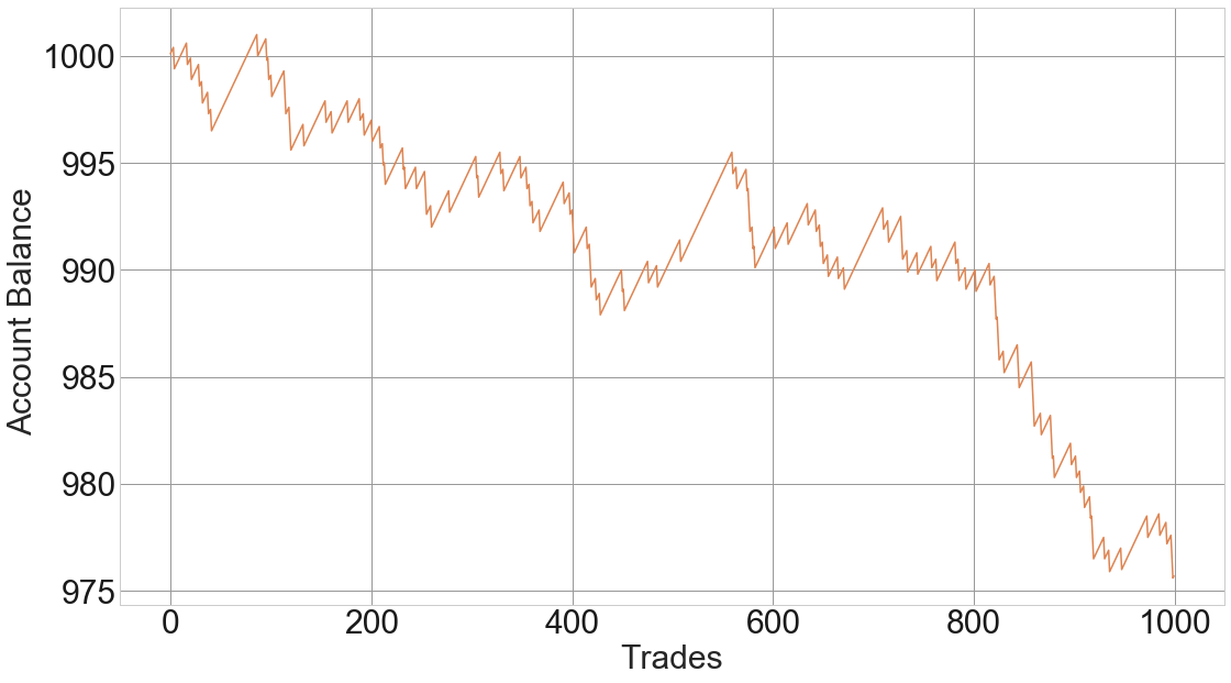
Fig 1 – Game with 90% winners where the player pays 10 dollars on losers and gains 1 dollar on gainers
This is a simulation of a game with 90% winners but with a reward-to-risk ratio of 0.1. Which means a loss wipes the value of ten previous winners.
Then, consider the next equity graph:
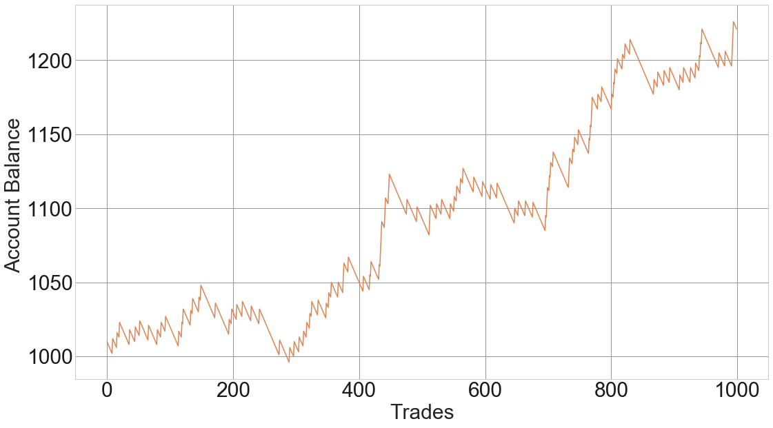
Fig 1 – Game with 10% winners where the player pays 1 dollar on losers and gains 10 dollars on gainers
A couple of interesting conclusions from the above graphs. One is that being right is unimportant, and two, that we don’t need to predict to be profitable. What we need is a proper method to assess the odds, and most importantly, define the reward-to-risk situation of the trade, utilizing the Expected Value concept,
By focusing on rewards instead of frequency of gainers, our strategy is protected against a momentary drop in the percent of winners.
The profitability rule
P > 1 / (1+ R) [1]
The equation above that tells the minimum percent winners needed for a strategy to be profitable if its average reward-to-risk ratio is R.
Of course, using [1], we could solve the problem of the minimum reward-to-risk ratio R required for a system with percent winners P.
R > (1-P)/P [2]
We can apply one of these formulas to a spreadsheet and get the following table, which shows the break-even points for reward-to-risk scenarios against the percent winners.

We can see that a high reward-to-risk factor is a terrific way to protect us against a losing streak. The higher the R, the better. Let’s suppose that R = 5xr where r is the risk. Under this scenario, we can be wrong four times for every winner and still be profitable.
Final words
It is tough to keep profitable a low reward-to-risk strategy because it is unlikely to maintain high rates of success over a long period.
If we can create strategies focused on reward-to-risk ratios beyond 2.5, forecasting is not an issue, as it only needs to be right more than 28.6% of the time.
We can build trading systems with Reward ratios as our main parameter, while the rest of them could just be considered improvements.
It is much more sound to build an analysis methodology that weighs both sides of the trade using the Expected value formula.
The real focus of a trader is to search and find low-risk opportunities, with low cost and high reward (showing positive Expected value).
Appendix: The Jupyter Notebook of the Game Simulator
%pylab inline
%load_ext Cython
from scipy import stats
import warnings
warnings.filterwarnings("ignore")
from scipy import stats, integrate
import matplotlib.pyplot as plt
import seaborn as sns
sns.set(color_codes=True)
import numpy as np
%%cython
import numpy as np
from matplotlib import pyplot as plt

# the computation of the account history. We use cython for faster results
# in the case of thousands of histories it matters.
# win: the amount gained per successful result ,
# Loss: the amount lost on failed results
# a game with reward to risk of 2 would result in win = 2, loss=1.
def pathplay(int nn, double win, double loss,double capital=100, double p=0.5):
    cdef double temp = capital
    a = np.random.binomial(1, p, nn)
    cdef int i=0
    rut=[]
    for n in a:
        if temp > capital/4: # definition of ruin as losing 75% of the initial capital.
            if n:
                temp = temp+win
            else:
                temp = temp-loss
        rut.append(temp)
    return rut
# The main algorithm.
arr= []
numpaths=1 # Nr of histories
mynn= 1000 # Number of trades/bets
capital = 1000 # Initial capital

# Creating the game path or paths in the case of several histories
for n in range(0,numpaths):
    pat =  pathplay(mynn, win= 1,loss =11, capital= cap, p = 90/100)
    arr.append(pat)

#Code to print the chart
with plt.style.context('seaborn-whitegrid'):
        fig, ax = plt.subplots(1, 1, figsize=(18, 10))
        plt.grid(b = True, which='major', color='0.6', linestyle='-')
        plt.xticks( color='k', size=30)
        plt.yticks( color='k', size=30)
        plt.ylabel('Account Balance ', fontsize=30)
        plt.xlabel('Trades', fontsize=30)
        line, = ax.plot([], [], lw=2)
        for pat in arr:
            plt.plot(range(0,mynn),pat)
        plt.show()
References:
More than you Know, Michael.J. Mauboussin
Fooled by randomness, Nassim. N. Taleb