Why you should Know The Normal Distribution
What is a Distribution
A Distribution comes from our need to measure and qualify objects or items when the potential number of elements is too large to evaluate one by one. It is hardly practical to have a record of all the heights, weights, races, clothes, and shoe sizes of every person. It is impossible to have a record of all possible stock or Forex pairs prices. Of course, we already have a historical record, but we cannot have a record of future prices. But we want and need information about these and other items.

Wouldn’t it be great to have valuable collective information about the properties of the data collection instead of an endless list of prices, heights, or weights?
Histograms
Let’s imagine that we are to record daily price changes from the current open to the previous day open. We could see that some days the price seldom moves while others there are larger and larger movements. Lets only plot ten possible ranges five on the positive side and five on the negative side, from zero to ±0.21, ± 0.2% – ±0.4%, and on toll ±0.8% -±1%. All changes bigger than 1% will be included in the ±0.8% – ±1% range.
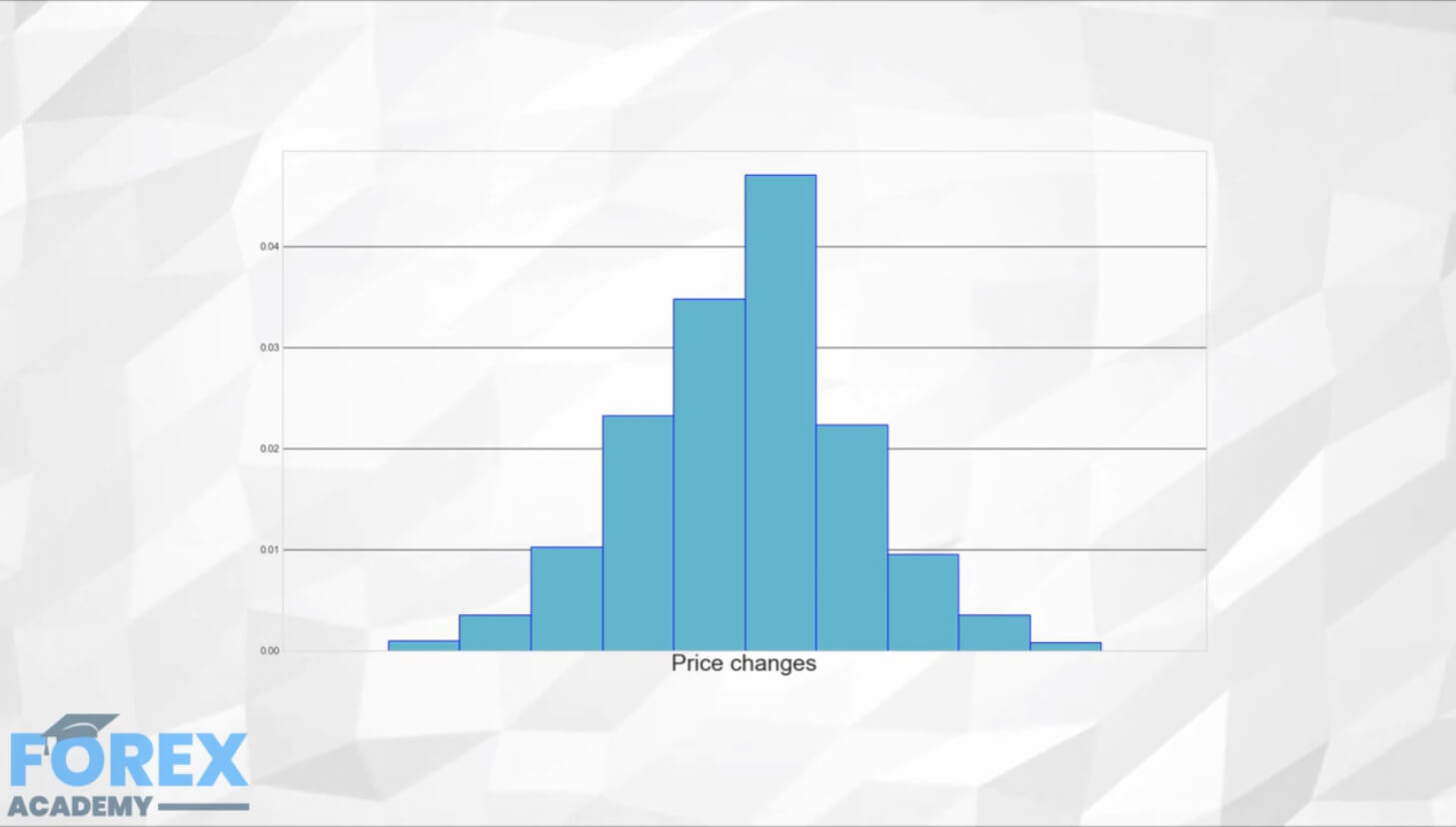
We have made a histogram of price changes. It is a very coarse approach to prices, but it shows useful information. We see that it is more common small changes than large changes, for instance.
We could refine it using more bins. This is how it looks using 40 bins.
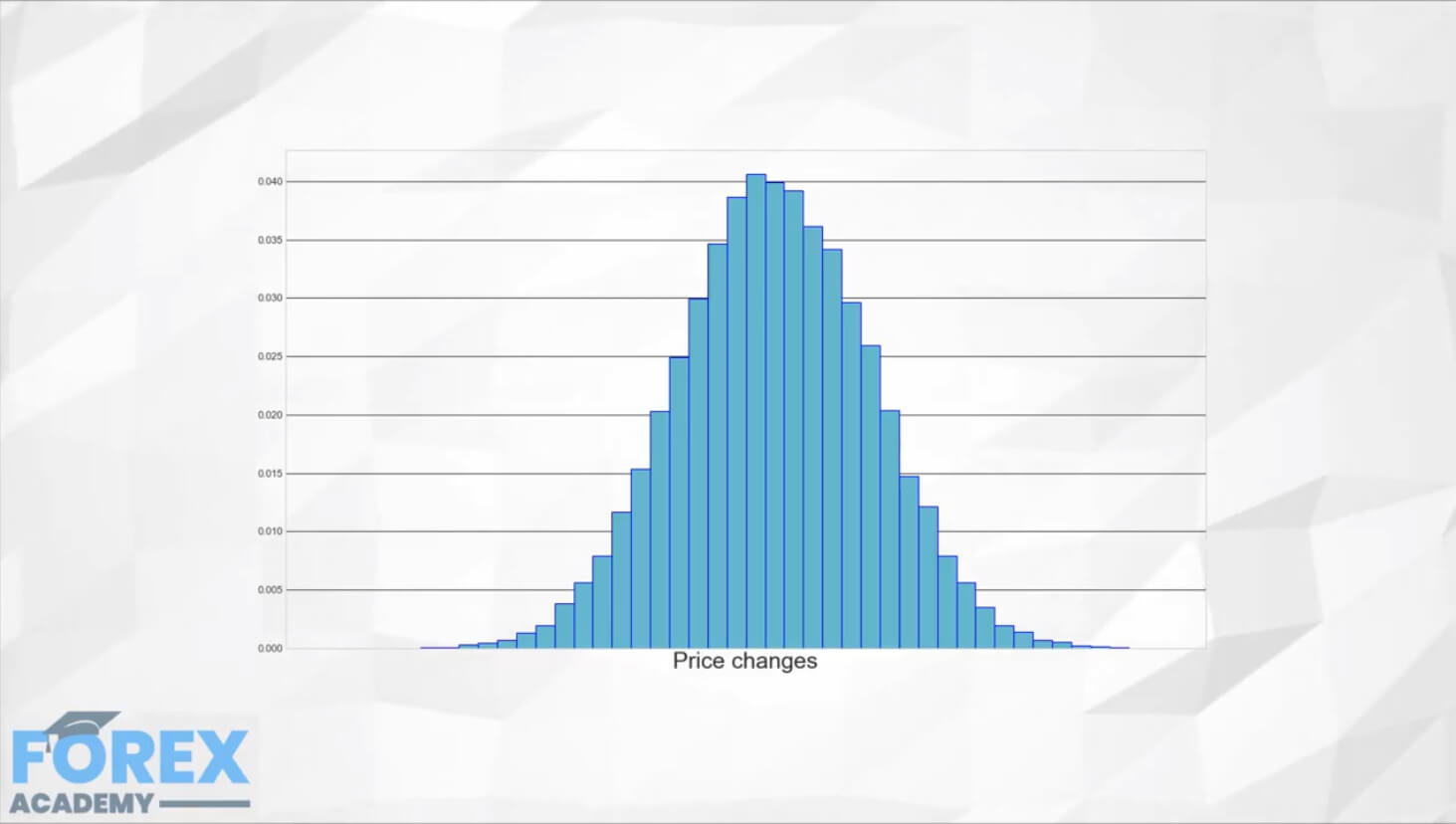
Using fewer bins, we can perceive the same distribution than using more bins. We lose information, but if we chose the bin distribution appropriately binning is quite convenient.
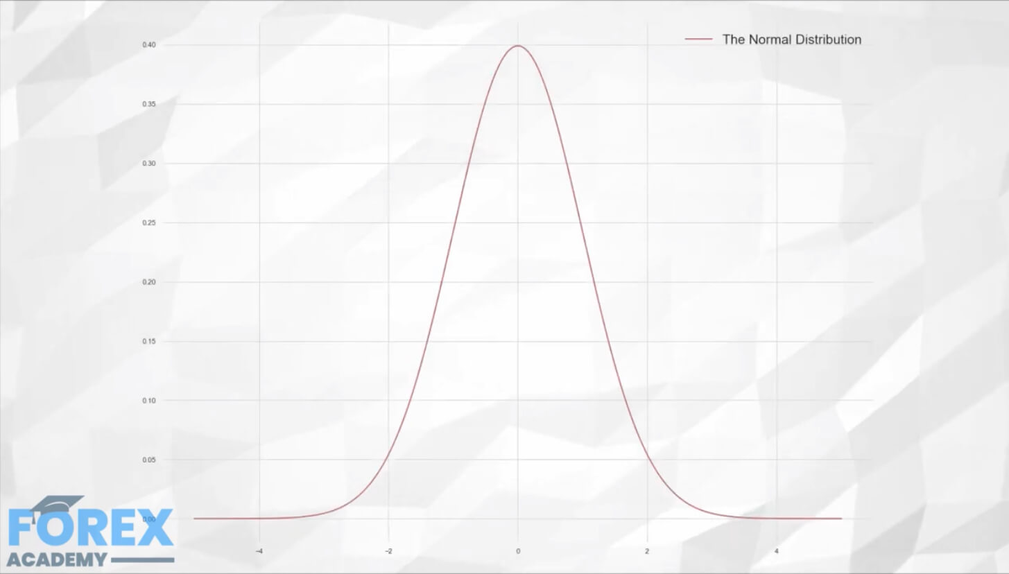
The Normal Distribution
Karl Friedrick Gauss was thought to discover the Normal Distribution, also called Gaussian Distribution, although 100 years earlier was described by Abraham d Moivre. Still, his discovery remained obscured until after Gauss published it. It is considered the most useful distribution in modeling due to the fact that many phenomena follow the Normal Distribution. Measures of height, weight, intelligence levels closely follow the normal distribution. Also, the Normal Distribution is the limiting form of other distribution types.
The Central Limit Theorem
One of the key statistical applications involving the Gaussian Distribution has to do with how the averages distribute. That is, if we take several random samples of a collection of data, the averages of the samples will approximate to a Normal Distribution, regardless of the distribution of the original data. This is very powerful because it allows us to generalize about future prices from the averages computed using samples of historical data.
Properties of the Normal Distribution
The Mean (M)
The most obvious measure of the Normal Distribution is its Average or Mean.
M = SUM ( All elements ) / N (the number of elements)
The mean tells us the most common value of the distribution. If the distribution were about prices, it would tell us the fair value of the asset.
The Standard Deviation (SD)
The other significative measure of the Normal Distribution is the Standard Deviation. Computing it is a bit more complicated than the average, but it is rather easy as well.
The standard deviation tells us how far from the center, on average, are its elements.
1.- We measure the distance of every individual component (dxi) from the mean
dxi = M – xi
2.- Since the differences may be positive or negative, we square this value to take away the sign, creating a collection of squared differences.
dxi2 = dxi^2
3.- We take the average of the squared differences. The result is called the variance (Var).
Var = SUM( dxi2)/ (N-1)
Wait? Why N-1? Well, that has to do with the fact we are dealing with samples, not the whole population. By dividing by N-1 will make the value less optimistic on short samples. As the sample size grows, the Sample Variance gets closer and closer to the population variance.
4.- We take the square root of the sample variance, and the result is the Standard Deviation
SD = √ Var
Normal Probabilities
Normal distribution probabilities
Now that we have our data (prices, trade returns, and so forth), we can use the normal distribution to extract useful information.
If the distribution, for instance, were the returns of our strategy, we would arrive at two main values: The average profit and the standard Deviation of the profits. What can that tell us about what to expect from our future returns?
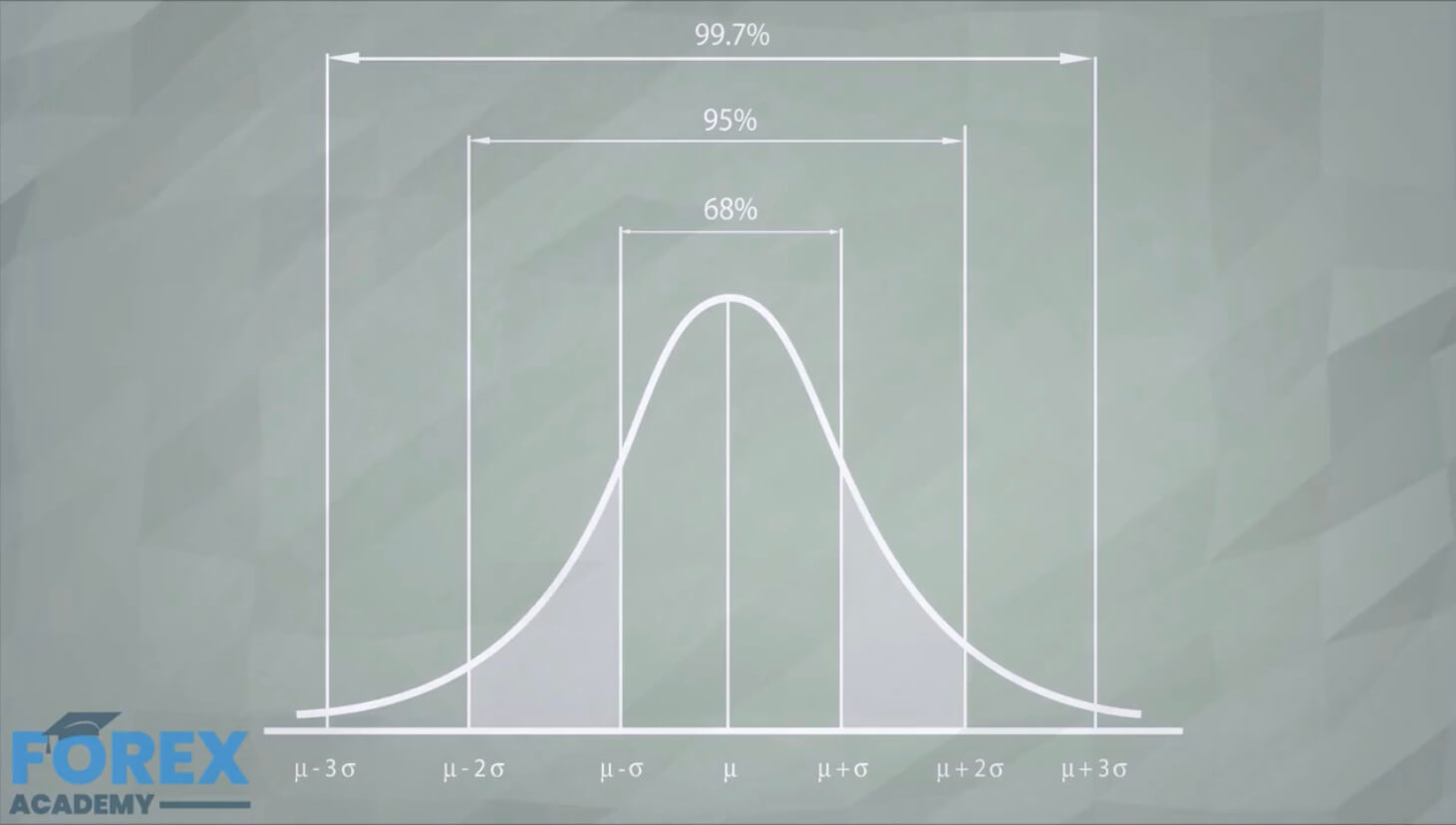
The Normal Distribution is well known, so we have how values are statistically distributed.
We know that 68.2% of the values lie within one SD from the mean, 95.4% of the values lie within 2SD, and 99.7% of them within 3SD.
Let’s say as an exercise that your mean gain is 100 dollars with an SD of 60. What can we expect from our future profits?
We can anticipate that
- 64% of the time, our returns will lie between 40 and 160 dollars,
- 13.6% of the time will be between -20 and +40 dollars,
- 13.6% between 150 and 210 dollars.
- 2.1% of the time your strategy will lose from 20 to 80 dollars
but also, - 2.1% of the time, you will get from 210 to 270 dollars.
As a caveat, Usually, the distribution of gains and losses is not normally distributed. Therefore we should not expect the percentages shown here. As homework, google about the Chevyshev’s inequality for a more general probability scaling.