Quantifying risk when trading has become one of the biggest concerns (or at least should be) as traders. The volatility, volatility of exchange rates, interest rates, etc. have made the study of risk increasingly important. In this article, we will show you how to use VaR and CVaR to assess your risk levels with a high degree of accuracy.

Another important issue that has enabled us to improve the study of risk, among those associated with our operation, has been the exponential increase in the computing capacity we currently have. Currently, as a trader, you have at your fingertips, from your laptop or smartphone, databases with all the necessary price history information for almost any financial asset you want to trade.
When developing a trading strategy or system we should not only focus on clearly establishing the rules for entering and leaving the market, but we should also objectively analyze the results of our trading system.
To achieve an objective analysis, a wide variety of metrics have been developed that evaluate different aspects of our operation. In this article, we will teach you to use two metrics based on risk control: Value at Risk (VaR) and Value at Risk (CVaR). These risk assessment measures have different methodologies and techniques for their estimation.
Before entering directly into the study of them, it is important that we have some basic concepts, such as what is financial risk and what are the types of risk.
What is Financial Risk?
In the investment context, the risk is the probability of loss due to events that can produce significant changes, and that affect a financial asset. Therefore, it is important that when we decide to make an investment, we identify and quantify the various types of risks to which we will be exposed when making the investment.
All investments carry an associated risk, but when we manage risk well we can find great opportunities for significant returns. Surely you’ve heard of “risk aversion”. Risk aversion refers to an investor’s attitude or preference to avoid financial uncertainty or risk. This leads him to invest in safer financial assets, even if they are less profitable.
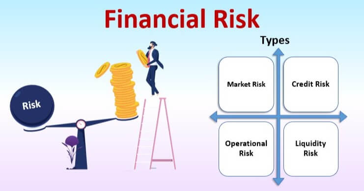
Types of Financial Risk
Although there are many risks in the investment world, financial risk can be classified into three main categories:
Market risk: this type of risk refers to loss risk arising from price movements of a financial asset or the market in general.
Credit risk: the inability of a party to respond with the obligations of an issue or with the strict terms of the issue (amount, interest, etc.), thus producing a loss for the counterparty.
Operational risk: This type of risk is defined as loss risk due to insufficiencies or failures of processes, personnel, and internal systems.
Now that we have clarified these basic concepts, let’s see what VaR and CVaR are all about.
Value at Risk (VaR)
Value at Risk is a statistical metric used to assess the risk of a given asset position or portfolio. VaR is the maximum expected loss, under normal market conditions, in a portfolio or trading system, with a probability (usually 1% or 5%) and a known time interval (usually a day, a week, or a month).
The VaR is measured through three variables: amount of loss, probability of such loss occurring (confidence level), and the time interval of occurrence. It is important to note that VaR does not seek to describe or predict worst-case scenarios, but rather to provide an estimate of the range of potential gains or losses.
Ways to calculate VaR
There are three main methodologies or approaches to calculating VaR:
Parametric method: when we calculate the VaR using the parametric method, we assume that profitability has a normal distribution and the portfolio is a linear function of the factors. For the parametric calculation, it is necessary to have the main statistical parameters (mean, variances, covariance, standard deviations, etc.) of the financial asset or portfolio that we are analyzing.
The formula for calculating VaR using the parametric method is as follows:
VaR = F * S * σ *
Where:
F = Value determined by the confidence level (also known as Z value).
S = Amount of portfolio or financial asset at current market prices.
σ = Standard deviation of asset returns.
t = Time horizon in which the VaR is to be calculated.
Historical simulation method: uses a large amount of historical data to estimate VaR, but makes no assumptions about probability distribution. One of the greatest limitations of this approach is that it assumes that all possible future changes in asset prices have already been observed in the past. The value of the VaR will depend on the source of the data and the size of the series (time frame of the data).
Monte-Carlo VaR Model: The calculation of VaR using the Monte-Carlo method is based on generating hundreds or thousands of hypothetical scenarios based on the series of initial data entered by the user. The accuracy of the VaR will depend on the number of scenarios we simulate, the higher the accuracy. The validation of the model is fundamental, for this it is recommended to carry out backtest tests to verify that the estimated VaR is verified with the historical series.
A practical example of how to calculate VaR:
I will do this by setting an example to calculate in VaR in actions to simplify calculations of pips and lots:
Suppose we have a portfolio composed of 1000 shares of the company ABC and the current price per share is 12$, the daily standard deviation is 1.8%. How can we calculate VaR with a 95% confidence level for a day?
The formula for calculating VaR is:
VaR = F * S * σ *
To calculate the value of F, we use the “DISTR.NORM.ESTAND.INV (probability)” function of the Excel spreadsheet.
F = DISTR.NORM.ESTAND.INV (confidence level) = DISTR.NORM.ESTAND.INV (95%) = 1.6448
S is the total amount invested in the portfolio and is calculated as follows:
S = share amount * market price = 1,000 shares * 12$ = 12,000$
The standard deviation σ is equal to 1.8%.
As we want to calculate the VaR for a day, then t = 1.

We replace the values in the VaR formula and have:
VaR = 1.6448 * $12
This VaR value tells us that the investor has a 95% confidence level that their investment will not lose more than $355.28 in a day.
What if we increase the level of confidence to 99%? In this case, the VaR would be:
VaR = 2.3263 * $12,000* 1.8% * = $502.48
This VaR value tells us that the investor has a 99% confidence level that their investment will not lose more than $502.48 in a day, or what’s the same, the probability of suffering losses greater than $502.48 during a day, is only 1%.
Advantages of VaR
Some very significant benefits of using VaR for the quantification of financial risk without the following:
-The VaR is a highly recognized standardized risk measure among traders and regulators. It has become a standard in the financial industry.
-It adds all the risk of an investment into a single number, making it very easy to assess the risk.
-It is probabilistic and provides us with useful information about the probabilities associated (confidence level) with a specific amount of losses (maximum loss).
-It can be applied to any kind of management and also allows you to compare risks of different portfolios regardless of their composition, whether fixed income or equities.
-The VaR allows you to add risks from different positions taking into account the way in which they correlate with each other, the different risk factors.
-It takes into account multiple risk factors and can focus not only on individual components but also on the overall risk of the entire portfolio.
-Because it is expressed in the loss of money (base currency; dollar, euro, etc.) it is simpler and easier to understand than other indicators that measure financial risk.
Disadvantages of VaR
But VaR, like any other metric used for trading systems, has its disadvantages:
-Generally depends on the quality of the historical data used for its calculation. If the data included is not accurate or correct, the VaR will be of little use.
-Although the interpretation of the values of VaR is very simple, some methods to calculate it can be very complicated and expensive, for example, the Monte Carlo method.
-It can generate a false sense of security in traders. Any measure of probability should not be construed as a certainty of what will happen. Remember that as traders, we only handle uncertainty scenarios never certainty scenarios, we do not make predictions.
-It does not calculate the amount of the expected loss remaining in the probability percentage.
Conditional Value at Risk (CVaR)
The conditional risk value (CVaR) is the mean of observations in the distribution queue, that is, below the VaR at the specified confidence level. Therefore CVaR is also known as expected deficit (Expected Shortfall, ES), AVaR (Average Value at Risk), or ETL (Expected Tail Loss).
The CVaR is the result of taking the weighted average of observations for which the loss exceeds the VaR. Therefore, the CVaR exceeds the VaR estimate, as it can quantify riskier situations, thus complementing the information provided by the VaR.
CVaR is used for the optimization of portfolios because it quantifies losses that exceed VaR and acts as an upper bound for VaR.

Properties of CVaR
CVaR stands out for having better mathematical properties than VaR, being a consistent measure of risk because it meets the criteria of:
Mono tonicity: If one financial asset performs better than another in any time horizon its risk is also lower.
Positive homogeneity: Refers to the proportionality between position size and risk.
Invariance to Transfers: By adding capital to a position your risk decreases in direct proportion to the capital added.
Sub-additivity: Asset diversification decreases the risk of a global position.
In summary, the most important message that CVaR is a consistent measure of risk is the following: the risk of two or more assets that make up a portfolio is less than the sum of the individual risks.
Interpretation of the conditional value at risk (CVaR)
The choice between CVaR and VaR is not always straightforward, since the conditional value at risk (CVaR) is derived from the value at risk (VaR). Generally, the use of CVaR rather than just VaR tends to lead to a more conservative approach in terms of risk exposure.
While VaR represents a maximum loss associated with a defined probability and time horizon, CVaR is the expected loss if you cross that worst-case threshold (maximum loss). In other words, CVaR quantifies the expected losses that occur beyond the VaR breakpoint.
As a rule, if an investment has maintained stability over time, the risk value could be sufficient for risk management in a portfolio that keeps the investment active. However, we must bear in mind that the less stable the investment, the greater the chances VaR will never display a complete image of the risk. In practice, trading systems rarely exceed VaR by a significant amount. However, more volatile systems may exhibit a CVaR many times larger than the VaR.
Finally, if we create a trading system and calculate your VaR, this VaR tells us what the maximum loss is with a certain level of confidence and time horizon. But if the loss is greater than VaR, how much should we expect to lose? This is where the conditional-at-risk value (CVaR) comes into play, which will tell us what the conditional average expected loss is if more is lost than the VaR.