Introduction
Globalization, the internet and also the massive use of computers have contributed to the worldwide spread of trading of all kinds: Stocks, futures, bonds, commodities, currencies. Even the weather forecast is traded!
In recent years, investors have turned their attention to the currency markets as a way to achieve their financial freedom. Forex is perceived as an easy place to achieve that goal. Trading currencies don’t know about bear markets. Currency pairs simply fluctuate driven by supply and demand in cycles of speculation-saturation, explained by behavioral economic science and game theory.
It looks straightforward: buy when a currency rises, sell once it falls.
However, this idyllic paradise has its own crocodiles that are required to be dealt with. The novel investor gets into this new territory armed with her own beliefs, that fitted well in his normal life but it’s utterly wrong when trading. But the main issues relating to underperformance lies inside the mind of the trader. Some say the market is rigged to fool most traders, however, the reality is that traders fool themselves. A shift in their core beliefs – and in the way they think- is critical for them to succeed.
The purpose of this, divided into three parts, is to boost awareness concerning three main issues the trader faces:
- The true knowledge about the nature of the trading environment
- The nature of risk and opportunity
- The key success factors when designing a system
The trading environment
Usually, people approach the study of the market environment by focusing mainly on market knowledge: Fundamentals, world news, central banks, meetings, interest rates, economic developments, etc. At that point, they interminably analyze currency technicalities: Overbought-oversold, trends, support-resistance, channels, moving averages, Fibonacci and so on.
They think that success is identified with that sort of information; that a trade has been positive because they were right on the market, and when it’s not is because they were wrong.
Huge amounts of paper and bytes have been spent in books and articles about those topics, yet there’s a concealed reality down there not yet uncovered, despite the fact that it’s the primary driver for the failure of the majority of traders (the other one is over-leverage and over-trading).
It’s evident that all traders are aware of the uncertainty of doing currency trading. Yet, except for individuals proficient about probability distributions, I am tempted to state that not a single person really knew what is this about, when she decided to trade currencies (at least not me, by the way).
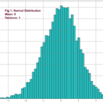
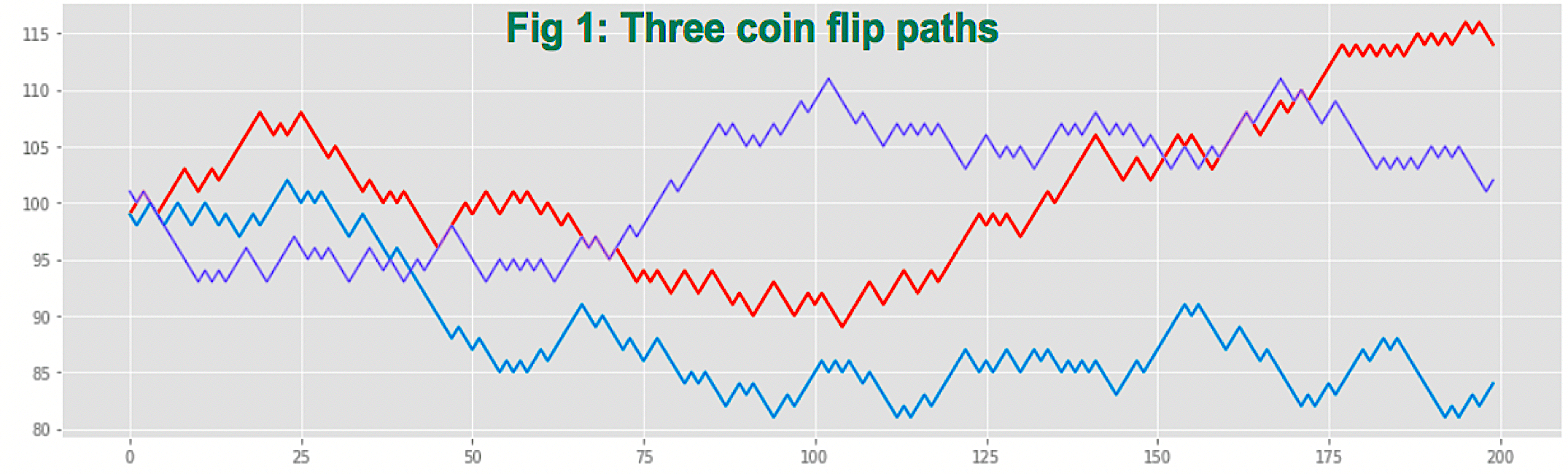
So, let’s begin. Everybody knows what a fair coin flip is, but what’s the balance of a fair coin flip game, starting 100€, after 100 flips if we earn 1€ when heads and lose 1€ when tails?
Many would say close to zero, and they might be right, but this is just one possible path: Fig 1: 100 flips of a fair coin flip game
There are other paths, for instance, this one that loses more than 20€:

Fig 2: 100 different fair coin flips
This second path seems taken from a totally different game, but the nature of the random processes is baffling, and usually fools us into believing those two graphs are made from different games (distributions) although they’re not.
If we do a graph with 1,000 different games, we’d observe this kind of image:

Fig 3: 1,000 paths of a fair coin flip 100 flips long
Below, a flip coin with a small handicap against the gambler:

Fig 4: 1,000 paths of an unfair coin flip
Finally, a coin flip game with a slight advantage for the player:

Fig 5: 1,000 paths of a coin flip with edge
And that’s the genuine nature of the beast. This figure above corresponds to a diffusion process and each path is called random walk. Diffusion processes happen in nature, likewise, for instance, as a billow of smoke ascending out from a cigarette or the spread of a droplet of watercolor in a glass filled with clean water.
Our first observation regarding fig 4 is that the mean of the smoke cloud drifts with negative slope, so after the 100 games, just about 1/3 of them are above its initial value; and we may observe that, even in the fair coin case, 50% of paths end in negative territory.
The game of a coin flip with an edge (fig 5) is the only one that’s a winner long term, although, short-term, it might be a losing game. In fact, before the first 20 flips, close to 50% of them are underwater, and at flip Nr. 100 about 35% of all paths end losing money.
If that game were a trading system, it would be a fairly good one, with a mean profit of 70% after 500 trades, but how many traders would hold it after 50 trades? My figure: only a 30% lucky traders. The rest would drop it out; even that long-term performance is good enough.
Below fig 6 shows a diffusion graph of 1500 bets of that game, roughly the number of trades a system that takes six daily bets produces in a year. We see that absolutely all paths end positive and the mean total profit is about 200%.

Fig 6: 1,000 paths of a coin flip with edge
By the way, the edge in this game is just a reward to risk ratio of 1.3:1, while keeping a fair coin flip.
Before going into explaining the psychological aspects of what we’ve seen so far, let me show you some observations we’ve learned so far, regarding this phenomena:
- The nature of the random environment fools the major part of the people
- There are unlucky paths: Having an edge is no guarantee for a trader’s success (short term).
- A casino game and the market, as well, collect money from endless hordes of gamblers with thin pockets and weak hands because they have no profitable system or stop trading his system before it could manifest its long-term edge.
- Casino owners know the math of gambling and protect themselves against volatility by diversification and a maximum allowed bet (only small gamblers allowed).
- By playing several uncorrelated paths at the same time, we could lower the overall risk, as does the casino owner, but we’d still need an edge and a proper psychological attitude.
- A system without edge is always a loser, long term.
The psychology of decisions taken under uncertainty
In 2002, Daniel Kahneman received the Nobel prize in economics “for having integrated insights from psychological research into economic science, especially concerning human judgment and decision-making under uncertainty.”
Dr.Kahneman did most of this work with Dr. Amos Tversky, who died in 1966. Their studies opened a new field of economics: Behavioural finance. They called it Prospect Theory and dealt with how investors make decisions under uncertainty and how they choose between alternatives.
One of the behaviors studied was loss aversion. Loss aversion shows the tendency for traders to feel more pain when taking a loss than the joy they feel when taking a profit.
Loss aversion has its complementary conduct: fear of regret. Investors don’t like to make mistakes. Both mechanisms combined are responsible for their compulsion to cut gains short and let loses run.
Another conduct taken from Prospect theory is that individuals believe in the law of small numbers: The tendency of people to infer long-term behavior using a small set of samples. They suffer from myopic loss aversion by assigning excessive significance to short-term losses, abandoning a beneficial long-term strategy because of suboptimal short-term behavior.
That’s the reason people gamble or trade until an unlucky losing streak happens to them, and the main reason casinos and the markets profit from people. Those who lose early, exit because they had depleted their pockets or their patience. Lucky winners will bet until a losing streak wipes their gains.
To abstain from falling into those traps, we should develop a strategy and get the strength and discipline to follow it, instead of looking too closely at results.
In Decision Traps, Russo and Schoemaker, have an illustrative approach to point to the process vs. outcomes dilemma:

Fig 7: Russo and Schoemaker: Process vs Outcomes.
Results are important and they are more easily evaluated and quantified than processes, but traders make the mistake to presume that good results come from good processes and bad results came from bad ones. As we saw here, this may be false, so we should concentrate on making our framework as robust as possible and focus on following our rules.
– A good decision is to follow our rules, even if the result is a loss
– A bad decision is not following our rules, even if the result is a winner.
The Nature of risk and opportunity
To help us in the task of exploring and finding a good trading system we’ll examine the features of risk and opportunity.
We’ll define risk as the amount of money we are willing to lose in order to get a profit. We may call it a cost instead of risk since it’s truly the cost of our operations. From now on, let’s call this cost R.
We define opportunity as a multiple of R. Of course, as good businesspeople, we expect that the opportunity is worth the risk, so we should value most those opportunities whose returns are higher than the risk involved. The higher, the better.
From the preceding section, we realize that the majority of new investors and traders tend to cut gains and let the losses run, in an attempt for their losses to turn into profits, caused by the need to be right. Therefore, they prefer a trading system that’s right most of the time to a system that’s wrong most of the time, without any other consideration.
The novel trader looks for ideas that could make their system right, endlessly back-testing and optimizing it. The issue is that its enhancements are focused in the wrong direction, and, likewise, most likely ending over-optimized. Thus, with almost certainty, the resulting system won’t perform well in practice on any aspect (expectancy, % gainers, R/r, robustness…)
The focus on probability is sound when the outcomes are symmetrical (Reward/risk =1); otherwise, we must take into account the size of the opportunity as well.
So, we’d like a frame of reference that helps us in our job. That frame will be achieved using, again, the assistance of our beloved diffusion cloud. The two parameters we’ll toy with will be: percent of gainers and also the Reward to risk (or Opportunity to cost ratio).
Since the goal of this exercise is to expel the misconceptions of the typical trader, we’ll use an extreme example: A winning system that’s right just 10% of the time, however with an R/r =10. It isn’t too pretty. It’s simply to point out that percent gainers don’t matter much:

Fig 8: A game with 10% winners, and R/r = 10.
Right! One 10xR winner overtakes nine losers.
The only downside employing a system with parameters like this is that there’s a 5% chance to experience 30 consecutive losses, something tough to swallow.
But there are five really bright ideas taken from this exercise:
- If you find an nxR opportunity you could fail on average n-1 times out of n and, still be profitable. Therefore, you only need to be right just one out of n times on an nX reward to risk opportunity.
- A higher nxR protects us against a drop in the percent of gainers of our system, making it more robust
- You don’t need to predict price movement to make money
- Repeat; You don’t need to predict prices to make money
- If you don’t have to predict, then the real money comes from exits, not entries.
- The search for higher R-multiples with decent winning chances is the primary goal when designing a trading system.
Below it’s a table with the break-even point winning rate against nxR

Fig 9: nxR vs. break-even point in % winners.
We should look at the reward ratio nxR as a kind of insurance against a potential drop in the percent of winners, and make sure our systems inherit that sort of safe protection. Finally, we must avoid nxR’s below 1.0, since it forces our system to percent winners higher than 50%, and that’s very difficult to attain combined with stop losses and normal trading indicators.
Now, I feel we all know far better what we should seek: Looking for what a good businessperson does: Good opportunities with reduced cost and a reasonable likelihood to happen.
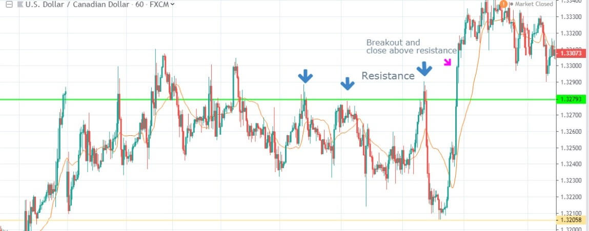
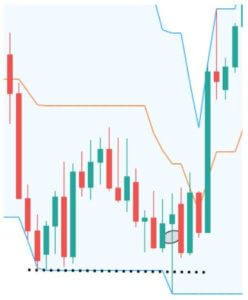
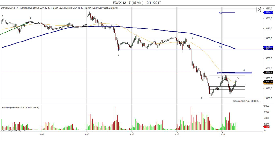
That’s what Dr. Van K. Tharp calls Low-risk ideas. A low-risk idea may be found simply by price location compared to some recent high, low or long-term moving average. As an example, let’s see this chart:

Fig 10: EUR/USD 15 min chart.
Here we make use of a triple bottom, suggested by three dojis, as a sign that there is a possible price turn, and we define our trigger as the price above the high of the latest doji. The stochastics in over-sold condition and crossing the 20-line to the upside is the second sign in favor of the hypothesis. There has a 3.71R profit on the table from entry to target, so the opportunity is there for us to pick.
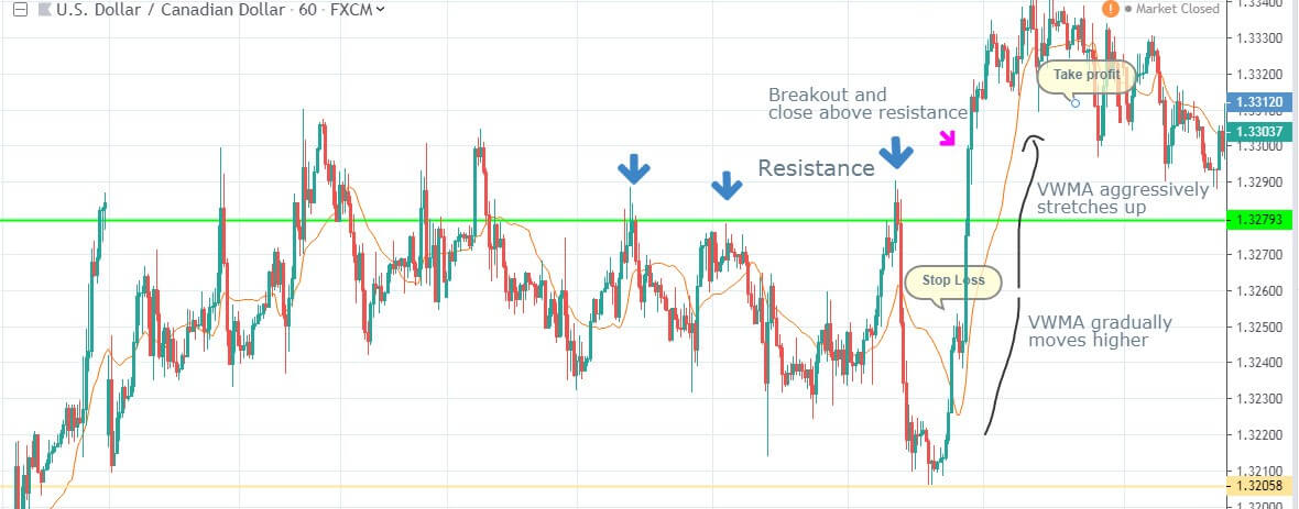
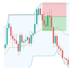
Here it is another example using a simple moving average 10-3 crossover, but taking only those signals with more than 2xR:

Fig 10b: USD/CAD 15 min chart. In green 2xR trades using MA x-overs. In red trades that don’t pass the 2xR condition
Those are simply examples. The main purpose is, there are lots of ideas on trading signals: support-resistance, MA crossovers, breakouts, MACD, Stochastics, channels, Candlestick patterns, double and triple tops and bottoms, ABC pattern etc. However, all those ought to be weighed against its R-multiple payoff before being taken. Another point to remember is that good exits and risk control are more important than entries.
Key success factors when designing a system
Yeo Keon Hee, in his book Peak Performance Forex Trading, defines the three most vital elements of successful trading:
- Establishing a well-defined trading system
- Developing a consistent way to control risk
- Having the discipline to respect all trading rules defined in point 1 and 2
Those three points are essential, however not unique. We need additional tasks to perfect our job and our results as traders:
- Using proper position sizing to help us achieve our objectives.
- Keeping a trading diary, with annotations of our feelings, beliefs, and errors, while trading.
- A trading record including position size, entry date, exit date, entry price, stop price, target price, exit price, the nxR planned, the nxR achieved; and optionally the max adverse excursion and max favorable excursion as well.
- A continuous improvement method: A systematic review task that periodically looks at our trading record and draws conclusions about our trading actions, errors, profit taking, stop placement etc. and apply corrections/improvements to the system.
First of all, let’s define what a system is:
Van K Tharp wrote an article [1] about the subject. There he stated that what most traders think is a trading system, he would call it a trading strategy.
To me, the major takeaway of Van K. Tharp’s view of what a system means is the idea that a system is some structure designed to accomplish some objectives. In reference to McDonald’s, as an example of a business system, he says “a system is something that is repeatable, simple enough to be run by a 16-year-old who might not be that bright, and works well enough to keep many people returning as customers”.
You can fully read this interesting article by clicking on the link [1] at the bottom of this document. Therefore I won’t expand more on this subject. If I discussed it, it was owing to the appealing thought of a system, as some structure designed to accomplish some goals that work mechanically or managed by people with average intelligence.
In this section, we won’t discuss details concerning entries, stop losses and exits- that’s a subject for other articles- however. We’ll examine the statistical properties of a sound system, and we’ll compare them with those from a bad system, so we could learn something about the way to advance in our pursuit.
Let’s begin by saying that in order to make sure the parameters of our system are representative of the entire universe of possibilities, we’d need an ample sample of trades taken from all possible scenarios that the system may encounter. Professionals test their systems using a multiyear database (10+ years as a minimum); however, an absolute minimum of 100 trades is a must, though it’s beyond the lowest size I might accept.
The mathematics of profitability
The main key feature of a sound system isn’t the percentage of gainers, but expectancy E (the expected value of trades).
Expectancy is the expected value of winners (E+) less the expected value of losers (E-)
(E+) = Sum(G)/(n+) x %Winners
(E-) = Sum(L)/(n-) x %Losers
Sum(G): The total dollar gains in our sample history, excluding losers
Sum(L): The total dollar losses in our sample history, excluding winners
(n+): The number of positive trades(Gainers)
(n-): The number of negative trades(Losers)
The expectancy E then is:
E = (E+) – (E-)
Similarly, we can compute
E = SUM(trade results)/n
Where n = total number of trades,
So E is the normalized mean or total results divided by the number of trades n.
If E is positive the system is good. The higher the E is, the better the system is, as well. If E is zero or negative, the system is a loser, even though the percentage of gainers was over 80%.
Another measure of goodness is the variation of results. Dr. Chis Anderson (main consultant for Dr. Van K. Tharp on his book about position sizing) explains that, for him, expectancy E is a measure of the non-random (or edge) part of the trade, and that we are able to determine if that edge is real or not, statistically.
From the trade list, we can also calculate the standard deviation of the set (STD).
From the trade list, we can also calculate the standard deviation of the set (STD). That can be done in Excel or by some other statistical package (Python, R, etc.). This is a measure of the variability of those results around the mean(E).
A ratio of E divided by the STD is a good metric of how big our edge is, relative to random variations. This can be coupled quite directly to how smooth the equity curve is.
Dr. Van K Tharp uses this measure to compute what he calls the System Quality Number (SQN)
SQN = 100 x E / STDEV
Dr. Anderson says he’s happy if the STDEV is five times smaller than E, that systems with those kind of figures show drawdown characteristics he can live with. That means SQN >= 2 are excellent systems.
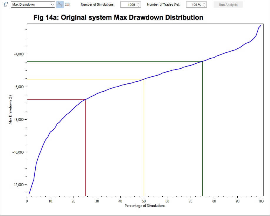
As an exercise about the way to progress from a lousy system up to a decent and quite usable one, let’s start by looking at the stats, and other interesting metrics, of a bad system- a real draft for a currencies system- and, next, tweak it to try improving its performance:
STATISTICS OF THE ORIGINAL SYSTEM:
Nr. of trades : 143.00
gainers : 58.74%
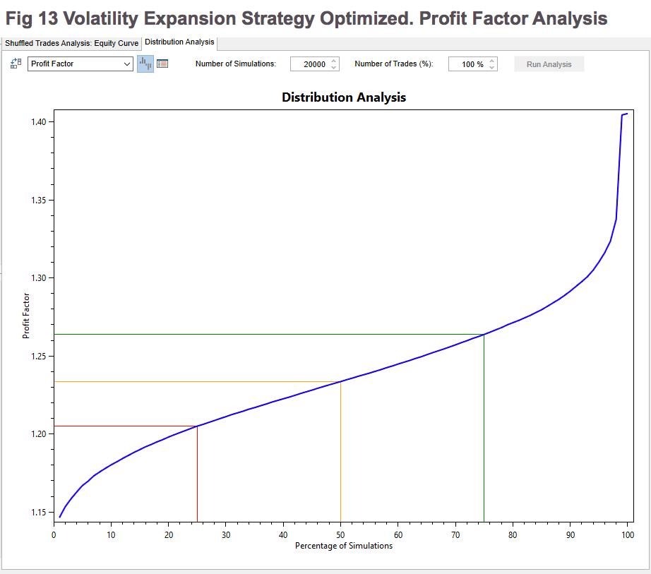
Profit Factor : 1.06
Mean nxR : 0.74
sample stats parameters:
mean(Expectancy) : 0.0228
Standard dev : 1.6351
VAN K THARP SQN : 0.1396
Our sample is 143 long, with 58.74% winners, but the mean nxR is just 0.74, therefore the combination of those two parameters results in E = 0.0228, or just 2,28 cents per dollar risked. SQN at 0.1396 shows it’s unsuitable to trade.
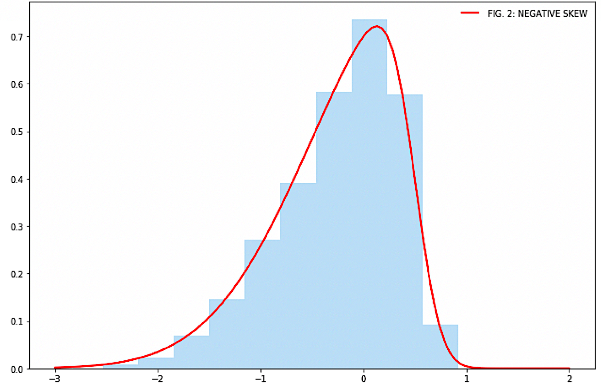
Let’s see the histogram of losses:

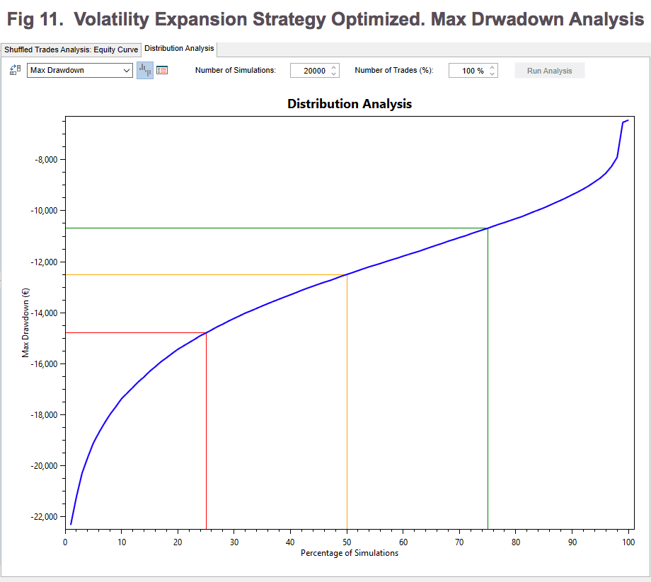
Fig 11: Histogram of R-losers (normalized to R=1)
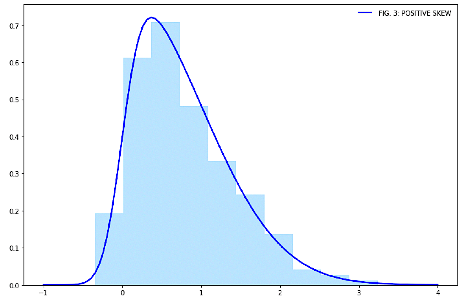
Original system probability of profits of x R-size

Fig 12: Histogram of R-Profits (normalized to R=1)
Diffusion cloud of 10,000 synthetic histories of the system:

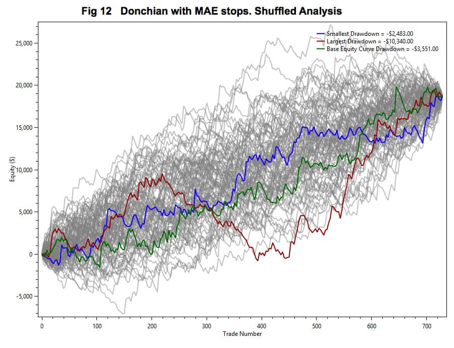
Fig 13: Original system: Diffusion cloud 10,000 histories of 1,000 trades.
Histogram of Expectancy of 10,000 synthetic histories:

Fig 14: Expectancy histogram of 10,000 histories of 1,000 trades. 50% of them are negative
We notice that the main source of information about what to improve lies in the histograms of losses and profits. There, we may note that we need to trim losses as a first measure. Also, the histogram of profits shows that there are too many trades with just a tinny profit. We don’t know what causes all this: Entries taken too early; too soon, or too late, on exits, or a combination of these factors. Therefore, we must examine trade by trade to find out that information and make the needed changes.
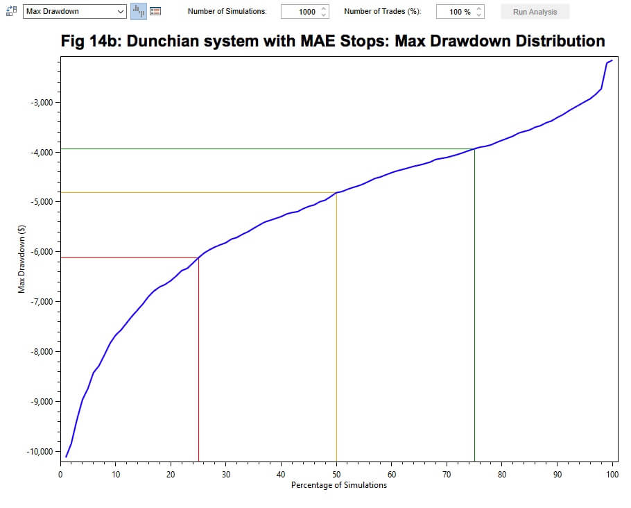
As a theoretical exercise, let’s assume we did that and, as a consequence of these modifications, we’ve reduced losses bigger than 2R by half and, also improved profits below 0.5R by two. The rest of the losses and profits remain unchanged. Let’s see the stats of the new system:
IMPROVED SYSTEM STATISTICS:
Nr. of trades             : 143.00 %
gainers                   : 58.74%
Profit Factor             : 1.99
mean nxR                  : 1.40

sample stats parameters:
mean(Expectancy)          : 0.4081
Standard dev              : 2.2007
VAN K THARP SQN           : 1.8546
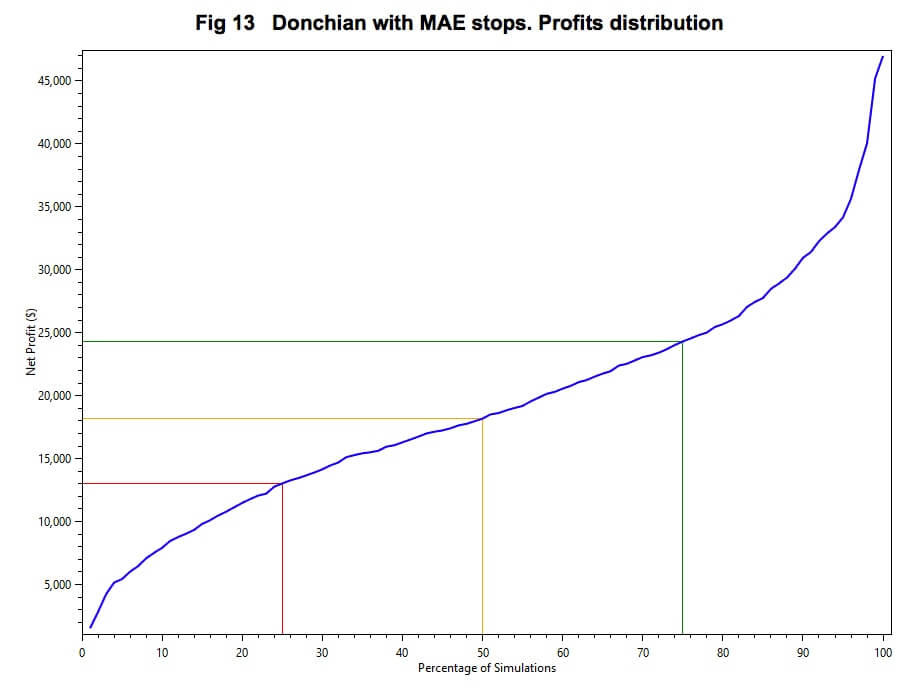
By doing this we’ve achieved an expectancy of 41 cents per dollar risked and an SQN of 1.53. It isn’t a perfect system, but it’s already usable to trade, even better than the average system:

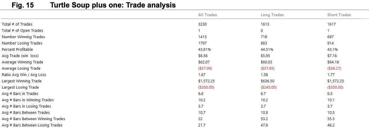
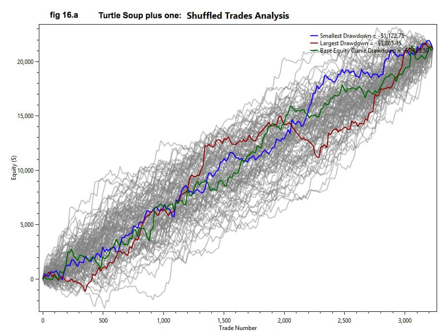
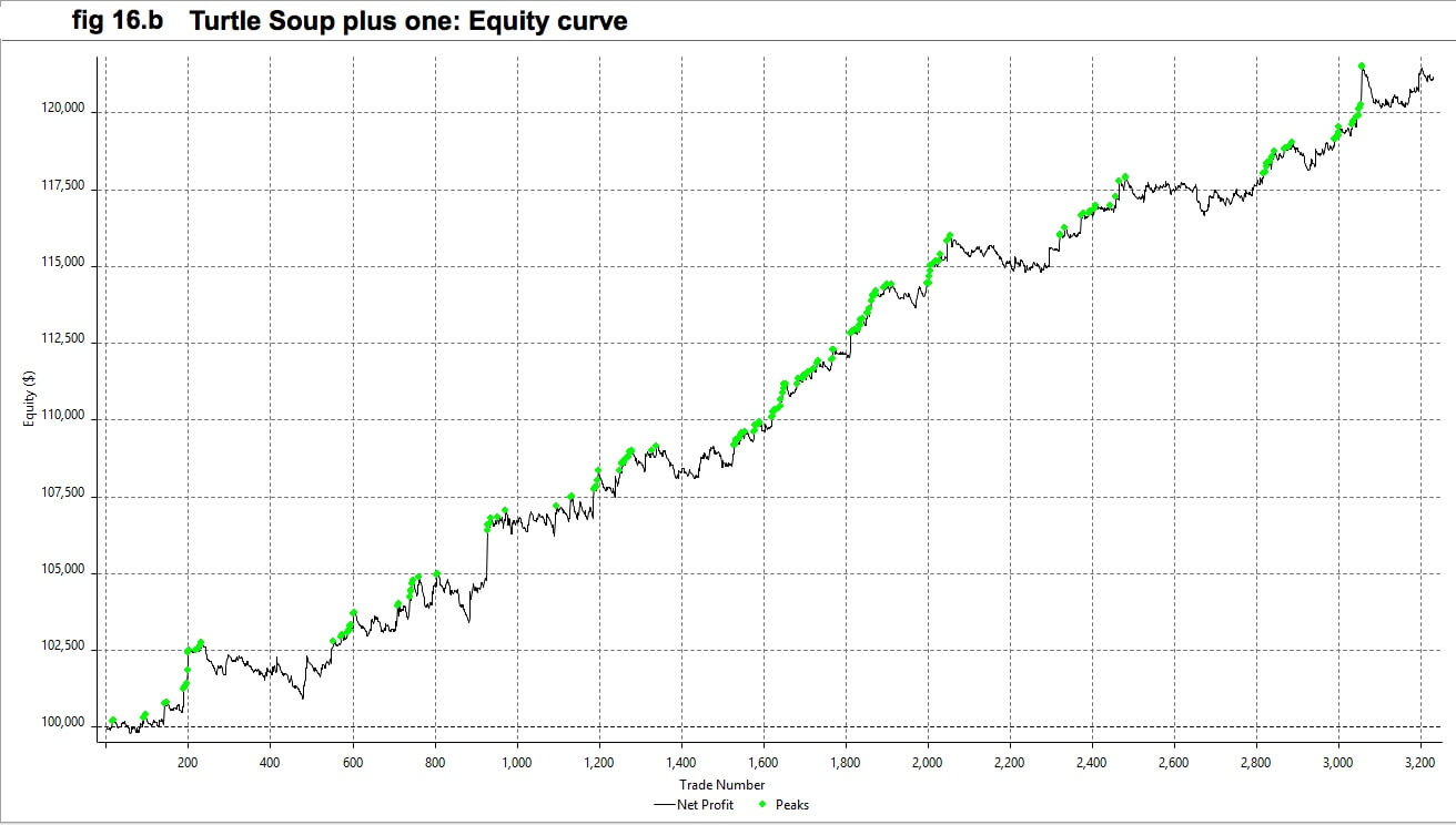
Fig 15: Improved system: Diffusion cloud 10,000 histories of 1,000 trades.
We may notice, also, on the histogram of Expectancies, below, that, besides owning a higher mean, all values of the distribution lie in positive territory. That’s an excellent sign of robustness and a good edge.

Fig 17: Improved system: Expectancy histogram of 10,000 histories of 1,000 trades.
There are other complementary data we can extract that reveal other aspects of the system, such those below:


Fig 17, for instance, shows that the system has a 40% chance of having 2 winners in a row, and 15% chance of 3 of them. Also, from fig 18, there’s a 60% chance of 2 loses in a row, 37% chance of 3 losers and 5% chance of a streak of 7 losers, so we must prepare ourselves against this eventuality by proper risk management.
Throughout this exercise, we’ve learned how to use our past trading information to analyze a system, decide what parts need to be modified, then perform the modifications, continue by testing it again using a new batch of results and observe if the new statistical data is sufficiently good to approve it for trading. Otherwise, a new round of modifications must be carried out.
Position Sizing
All figures and stats we’ve seen until now belong to an R-normalized system: It trades just a unity of risk per trade, without any position sizing strategy at all. That is needed to characterize the system properly. But the real value of a framework that allows this type of measurements is to use it as a scenario planning to experiment with different position sizing strategies.
We should remember, a system is a structure to achieve specific goals.
And position size is the method that helps us to achieve the financial goal of that system, at a determined financial maximum risk.
As an exercise, Let’s look at what this system may accomplish by maximizing position size without regard for risk (besides not going broke).
We’ll do it using Ralf Vince’s optimal f: The optimal fraction of our running capital. The computation of optimal f for this system was done using a Python script over 10,000 synthetic histories and resulted in a mean Opt f = 22%. To be on the safe side, we’ll use 75% of this value. That means the system will bet 16.77% of the running capital on every trade.
The result of the diffusion cloud will be shown in semi-log scale to make it fit the graph:

Fig 19: Improved system: Diffusion cloud traded with Optimal f. y log scale.
Below the probability curve of the log of profits, on a starting 10,000€ account, after 1000 trades:
Starting capital   :  1.0 e+4
Mean ending Capital:  2.54013596e+10
Min  ending Capital:  4.20930083e+02
Max  ending Capital:  3.94680594e+18
We see that there is 50% chance that our capital ends at 25,400 million euro (2.54 e+10) after 1000 trades, and a small chance of that figure is 3+ digits higher. Of course, the market will stop delivering profits much early than this. The purpose of the exercise is to show the power of compounding using position sizing.
Let’s see the drawdown curve of this positioning strategy:

We observe there’s 80% chance our max drawdown being more than 75% and 20% chance of it being 90%, so this kind of roller-coaster isn’t for the faint heart!
Before finishing with this scenario, let’s look at a final graph:

This graph shows the probability to reach 10x our initial capital after n trades. For this system, we observe that there’s a 25% chance (one out of 4 paths) that we could reach 10X in less than 80 trades and a 50% chance this happens in less than 150 trades.
That shows an important property of the optimal f strategy: Optimal f is the fastest way to grow a portfolio. The closer we approach optimal f the faster it grows. But as position size goes beyond the optimal fraction the risk keeps increasing but the profit diminishes, so there’s no incentive to trade beyond that point.
That property may suggest ideas about an alternative use the use of optimal f. If you think about a bit, surely, you’ll find some of them.
My goal with this exercise was to show that any average system can achieve any desirable objective.
Now let’s do another useful exercise. Let’s compute the fraction that fulfills a given objective limited by a given drawdown.
Let’s do a position sizing strategy for the faint-heart trader. He doesn’t wish more than 10% drawdown, accepting a 5% probability that drawdown goes to 15%. His primary concern is the risk, so he takes what the system could deliver within that small risk.
To find this sweet spot we need to try several sizes on our simulator using different fractions until that spot is reached. After a couple of trials, we find that the right amount for this system is to trade 1% of the running balance on each trade. Here we assumed that no other systems are used, and just one trade at a time. If several positions are needed, then the portfolio should be divided, or, alternatively, we must compute the characteristics of all systems combined.
Below, the main figures of the resulting system:

Starting Capital   :  10,000
Mean ending Capital:  45,508
Min  ending Capital:  13,406
Max  ending Capital:  177,833

Mean drawdown: 9.58%
Max drawdown: 25.98%
Min drawdown: 4.13%
We observe, the system performs quite well for such small drawdown, with 100% of all paths more than doubling the capital, and a mean return of 455% after 1,000 trades.

Finally, the figures for a bold trader who is willing to risk 30% of its capital, with just a small chance of more than 40%, are shown below.

Starting Capital   :  10,000
Mean ending Capital:  710,455
Min  ending Capital:  19,890
Max  ending Capital:  37,924,312

Mean drawdown: 26.43%
Max drawdown: 60.52%
Min drawdown: 11.97%
We observe that this positioning size is about 2.5 times riskier than the previous one. In the more conservative position sizing, we have a 5% chance of 15% max drawdown, while this one has a 5% chance of about 38% drawdown. But on returns we go from a mean ending capital of 45,500€ to a mean ending capital of 710,455€, surpassing by more than 10 times the returns of the first strategy.
This is common in position sizing compounding. Drawdowns grow arithmetically, returns grow geometrically.
Summary
Throughout this document, we’ve learned quite a bit about the three main aspects of trading.
Let’s summarize:
Nature of the trading environment
- The nature of the random environment fools a majority of the people
- New traders want to be right so they cut their profits while hanging on their losses
- New traders are psychologically affected by the law of small numbers, and fail because they believe in the law of small numbers instead of being confident by the long-term edge of their system.
- Having an edge is no guarantee for a trader’s success (short term) of you don’t have an edge and the discipline to follow your system.
- By splitting the risk into several uncorrelated paths at the same time, we could lower the overall risk
- A system without edge is always a loser long term.
The nature of risk and opportunity
- If we look for nxR opportunities, we just need to succeed once every n trades be profitable.
- A system with higher nxR is protected against a drop in the percent of gainers of our system, making it more robust.
- We don’t need to predict price movement to make money.
- If we don’t need to predict, then real money comes from exits, not from entries.
- The search for higher R-multiples with decent winning chances is the primary goal when designing a trading system.
Key factors to look when developing a system
- A system is a structure designed to accomplish specific goals that work automatically.
- The three most vital elements of successful trading:
- Establishing a well-defined trading system
- Developing a consistent way of controlling risk
- Having the discipline to respect all trading rules defined in point 1 and 2
- Using proper position sizing helps us achieve our objectives.
- Keeping a trading diary, with annotations of our feelings, beliefs, and errors, while trading.
- It’s essential to keep a trading record
- We need a continuous improvement method: A systematic review task that periodically looks at our trading records and draws conclusions about our trading actions, errors, profit-taking, stop placement, etc. and apply corrections/improvements to the system.
- Position sizing is the tool to help us achieve our specific objectives about profits and risk.
References
[
1]
http://www.stockbangladesh.com/blog/what-is-a-trading-system-by-van-k-tharp/
Recommended readings:
Trade your way to your financial freedom, Van K. Tharp
Peak performance Forex Trading, Yeo, Keong Hee


 The daily chart is looking bearish as the Bitcoins price failed to create a higher high and is now 6823$. Not much has changed since yesterday, expect that the price slightly rose by 1,84%.


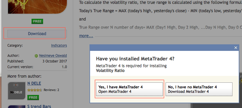
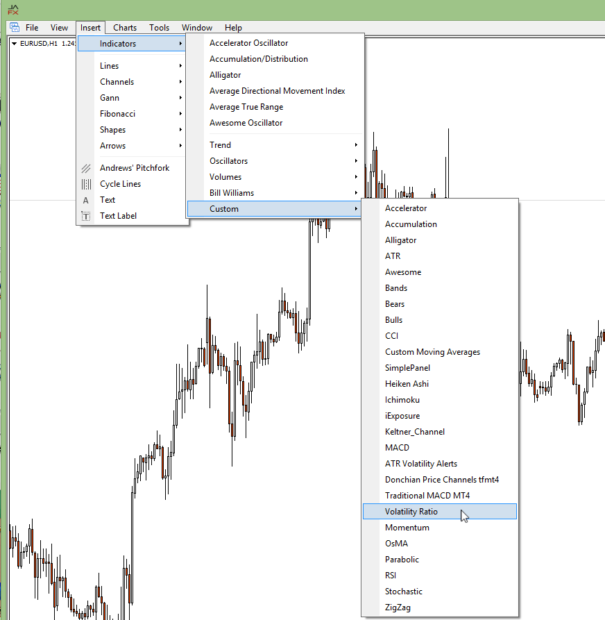


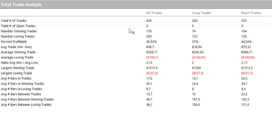
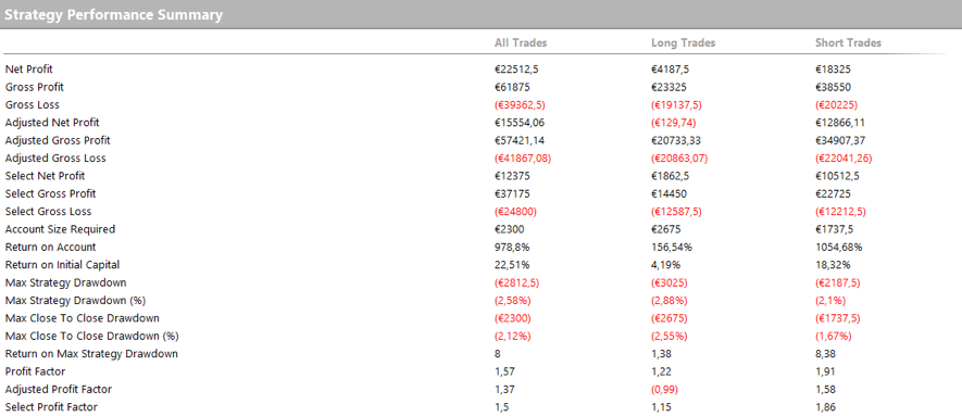
 Forex traders usually get MT4 for free when opening a trading account, and MT4 includes what it calls a “strategy tester” which is accessible by clicking a magnifying glass button or Ctrl-R.


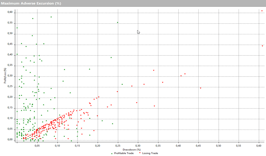
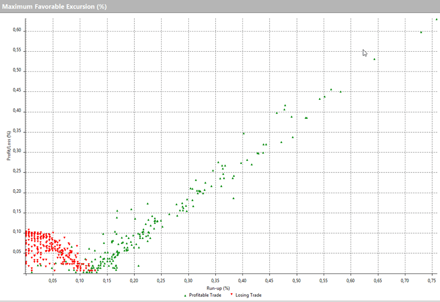
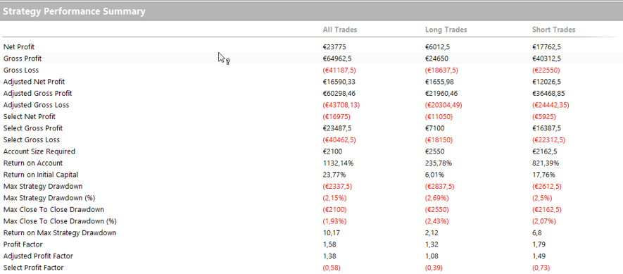
 Based on the above results, we set the stop at 0.105% of retraction, and now it looks like this.
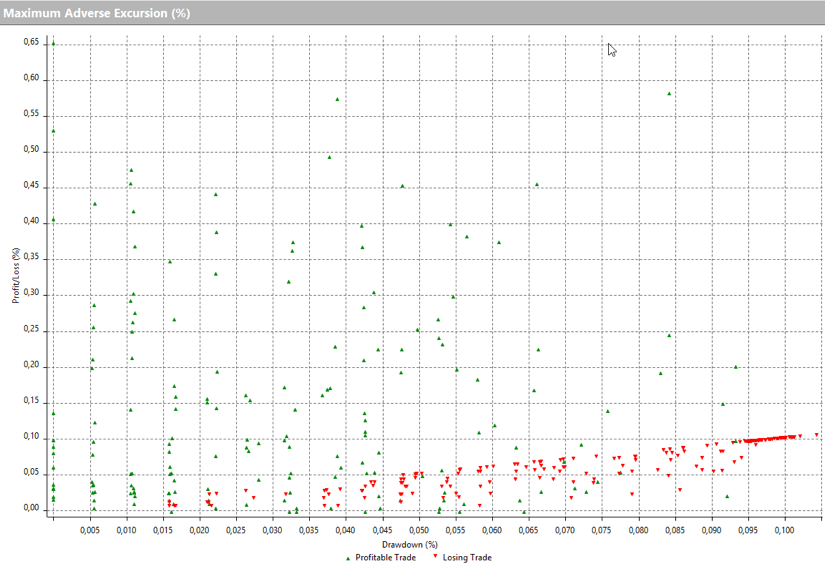
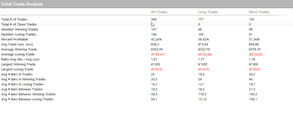
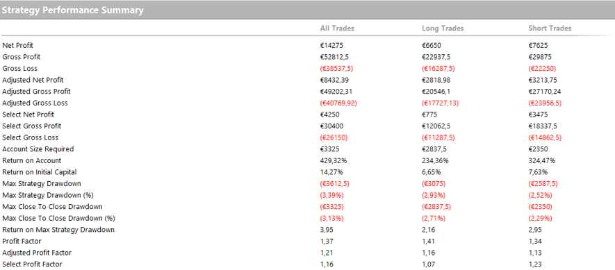
 The statistics are as follows:
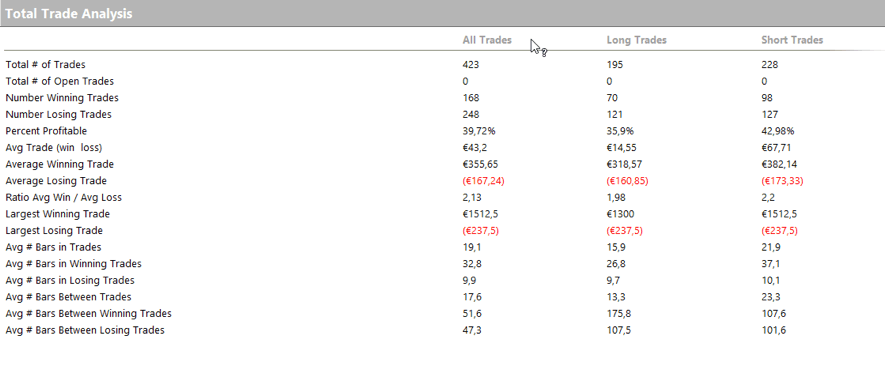

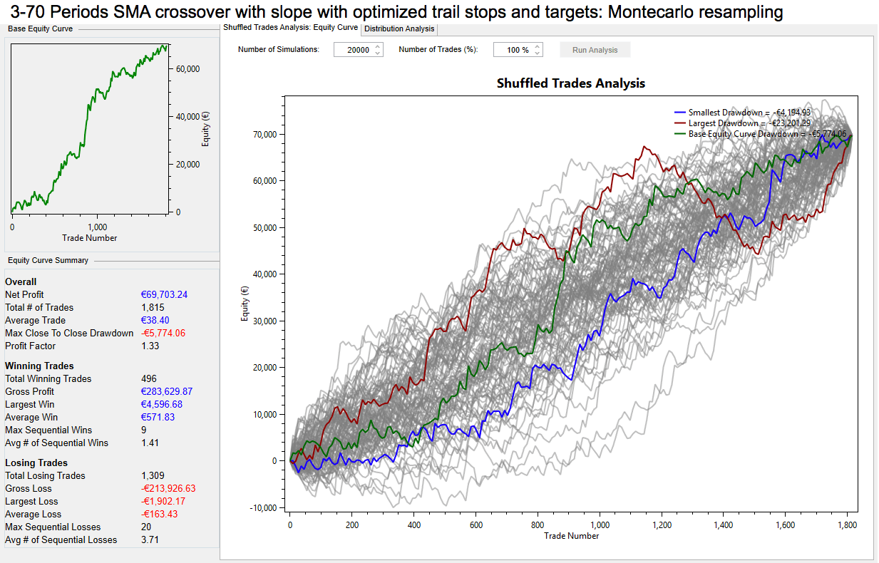
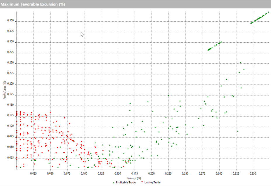
 Now to advance the robustness of the system, let’s look at the Maximum Favorable Excursion (MFE) by looking at the following graph.
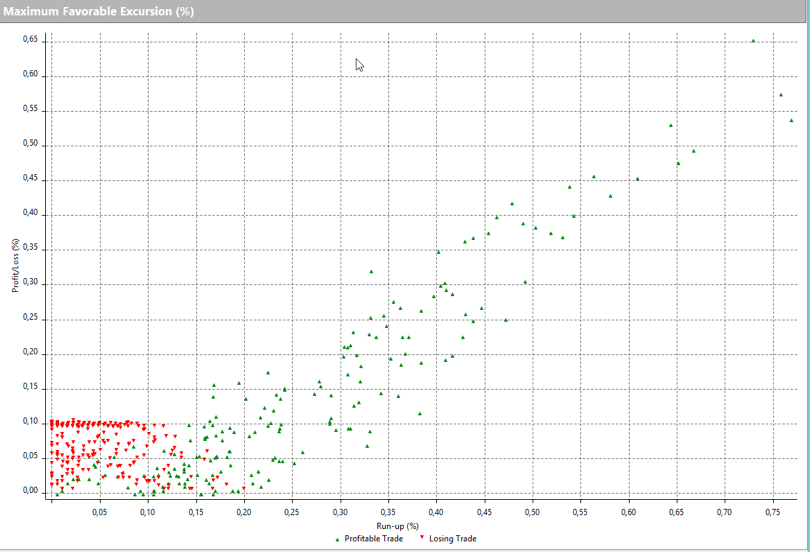


