Categories
Forex Courses on Demand

Introduction To Elliot Wave Theory – Accurately Predicting Forex trends

Hello, and welcome to this latest edition of courses on demand, brought to you by Forex Dot Academy. So, in this course, we’ll be looking to provide you with a pretty comprehensive introduction to what’s called Elliot wave theory. So, just before we begin, there is, of course, inherent risks involved in trading the financial markets. So, please do take a brief moment to familiarise yourself with our disclaimer, if you do need to stop or pause this recording do feel free to do.

So, okay, let’s start with a very brief webinar outline we’ll start by giving you an introduction to Elliot wave theory! We will explain the origin of Elliot wave theory, and a little bit about the creator, and how this whole theory came about. Then we’ll have a look at the actual Elliot wave theory itself, and it’s referred to as the five-wave pattern. Now,  within that there is what’s called impulsive waves we’ll have a look at those we’ll have we’ll have a look at corrective waves, and the fact that these wave patterns do repeat themselves, and of course there are variances on these waves as well. So, you can have a situation where you can have a series of waves even within waves. So, all this will become very transparent very shortly, and we’ll have a look at Elliot wave theory in practice as well. So, you can see it on a price chart, and we’ll finish by just looking at some of the difficulties that traders can have when applying Elliot wave theory okay. So, let’s start with an introduction to Elliot wave theory then. So, what’s important to be aware of it is that Ralph Nelson Elliot, and I put a picture of him up on the screen, and developed the Elliot wave theory in the late 1920s. Now,  he believed that the markets who many believed behave in a very erratic manner actually trades in more of a repetitive cycle. So, to give you a bit of background behind Ralph Nelson Elliot he was born 1871, and he died in 1948 he was a US Treasury accountant. Now,  in his 50s he began to study stock market data looking at price action, and he observed that stock market prices trend, and reverse in recognisable patterns, and this of course then was able to give birth to his Elliot wave theory and. So, to just encapsulate what the Elliot wave theory is. Now,  this is a theory which suggests that market moves in clearly defined sequences of highs, and lows in a very repetitive manner and. So, the Elliot wave theory studies the movements of these sequences. So, at this point, I’d like to bring up just a fairly generic price chart, and because there is a couple of things before we begin that we would just need to point out to you. So, firstly it’s just important to know that our to recognise Elliott wave theory as a technical tool effectively which is used exclusively by technical traders, and what it sets out to do is also as well, it’s important to embrace the fact that markets are continually prone to trending, and reversing am I even in a linear fashion, and this particular chart is just a typical example it is a US dollar monthly price chart but what you can see is that this chart can move in a particular pattern either to the downside or to the upside. So, it can go through periods of trending lower in a very repetitive fashion, and of course, you can get slight reversals of that where you’re getting pullbacks in price action off those levels, and then you can reestablish these trend patterns. So, this is what Elliot was interested in is identifying, and trying to understand what is going on with these market movements, and of course the same applies to the upside you can go through periods of price action, and of course, be able to identify the pullbacks as well.

So these markets constantly go through periods of trending either to the upside or to the downside. So, you could have this just trending market on a number of occasions trending to the downside, and therein lies potential opportunities for your bears to look to the seller’s market, and you also get these opportunities to buy these markets as well, for your Bulls. So, markets never move in a linear fashion; they do not move in straight lines. So, we have to acknowledge that markets move in trends, and they reverse, and then they can move in trends as well, they can go through also periods of consolidation and. So, this is just the nature of the way that the markets operate. So, that’s just a little bit about just a brief introduction to Elliott Wave, because we’ll explain it. Now,  in considerable more detail, and we’ll start with the basic principle of the Elliot wave theory is the five-wave pattern. Now,  what this suggests is any major movement will unfold in a pattern of five waves, and in turn will be corrected via a pattern of three waves going in the opposite direction. So, just imagine this diagram here in the middle of your screen represents price action, and the movement of price, and we can identify that this market creates a high price point number one you can see it then pulls back to two it moves higher to three it then pulls back again to number four, and then we this market seems to peak at the fifth wave which is the fifth impulse pushing prices higher then look what happens, because the five-wave movement can be split into two distinctive segments, and we look at each segment very carefully but what happens after we see a price point they’re on-screen at five at the fifth wave we can then see that the market makes a reverses, and it makes a low at Point, and it then tries to push higher fails to make a new high, and makes a high at point B, and of course makes a third wave pattern to the downside in the opposite direction of the initial move. So, this is your impulse, and this is your correction. So, what Elliott would do, and he’ll be analysing a lot of price data is he’d be identifying these patterns existing in the markets either on the impulse side, and then looking at the correction side, and what he suggested was there’ll be interesting opportunities at these points, if you can identify them for opportunities to buy these markets at these levels and, if you can identify one three, and five what it will do for traders is potentially give them an opportunity in this case to sell the market, and benefit from this reduction or pullback in price action, and you can use this five-wave pattern to do that followed by a three-wave correction, and that is the basic premise behind Elliott’s wave theory. So, we will apply this technically in a chart very shortly, but I do want to just focus a little bit more on the impulse wave, and it’s being able to identify these one two five waves which we’ve just highlighted there in the box. So, this trend phase is known as the impulse phase. So, we’re getting impulses to the upside on again on numerous occasions, and I shall just briefly change the -colour. So, we’re getting these impulses pushing prices higher from these points on a price chart, and this is the end of the essence of the impulsive segment of this particular wave. So, we’re getting that trending price action pushing prices higher. So, this is the numbered phase. So, the first five phases are actually broken down as the numbered phase.

So, you’re looking for one two three four five-wave patterns on a chart, and an impulsive segment one two five is itself constructed as a series of five waves of which one three, and five impulses are of a minor degree. So, we’re experiencing a nice sizeable move in price action from the low to the outright high, and we’re able to identify with our understanding of this impulsive segment or the impulse waves, and we’re identifying potentially tradable opportunities within that okay. So, that’s just a little bit about the impulse wave. So, moving on to. Now,  the corrective wave, and which we’re again going to look at the same representation of price action but actually there’s a little bit more to the corrective segment the corrective part of the corrective wave and elements of this particular Elliot wave theory. So, trends move in a series of peaks, and troughs or highs, and lows, and other technical analysts would refer to one as a high would refer to as a low would refer to three as a higher high will doing a slightly bigger would refer to for as a higher low. So, really it’s just a chain a slight change in terminology, and this number five would be a higher high once more. So, as price drives to the upside in phase one up to phase three, and up to phase five this the corrective wave actually focuses on the parts of the wave which result in prices pulling back. So, we also have the lettered phase as well, is known as the corrective segment, and has always counted in threes. So, whereas we’re looking for five waves to the upside, and we would also be looking, if you’re applying Elliot wave theory three waves to the downside in this particular example, and they’re always counted in threes, and to differentiate between the impulsive and the corrective wave we’re. Now,  looking at ABC in terms of a price move. So, highlighting wave number two, and number four of the impulsive phase are also corrective waves, because those are the lows that are created, because of a correction of price, and that’s just means we get a pullback to that to that low, and that creates our wave number two, and wave number four. So, once we’ve satisfied that we see wave 1 then we see wave 2 we see a push higher at wave 3 we see the pullback at bay 4 then this constitutes Elliot the Elliot wave theory, and where you make a higher at 5, and then you see the reversal in that price action or the corrective second or the corrective wave. So, in addition to that waves 2, and 4 as a result of the impulsive phase are also corrective waves wave 2 corrects wave 1. So, we’re getting this push higher. So, this lower here correct the price action, because we don’t see price action moving in a linear fashion, and it does move in this impulse to the upside followed by a pullback followed by a further impulse followed by a pullback. So, it’s just following that as a narrative but being able to visually identify it on a price chart we have a look at some price charts very shortly to show you this in a little bit more detail. So, just be aware that wave 2 corrects wave 1, and of course wave number 4 corrects wave 3. So, the correction always comes after the impulse, and ABC is the corrective phase of waves 1 to 5. So, this is the corrective segment. Now,  wave 2, and 4 is the individual correction, and then we enter once the price peak at 5, we then enter the corrective segment creating an A, B, and C corrective wave in this example. Now,  other tools can be used to help identifying where a market will pull back, for example, at fib levels. So, you know those that that trade the market using technical indicators that may use fib levels they might draw a fib from the low the recent low to the recent high, and they might be able to gauge where this price action will actually pull back to even at Point a the first corrective wave or Point C which is the second corrective wave pushing lower. So, that can just present with opportunities for traders to actually look to engage with the fib, and there’s obviously many other trading indicators as well, which can be used in a similar fashion that can support the understanding as well, of Elliot wave theory.

So, moving on then to the fact that what’s important, when  you understand the complete structure, and you identify you can identify these five-wave patterns, and you can see them in every chart in some capacity it’s important to understand that you know week you can experience with a very volatile moving chart that waves can repeat themselves on multiple occasions and. So, you can get these smaller waves existing, and these you get your 5 wave impulse followed by your ABC wave correction, and this has the tendency to repeat itself on many occasions especially, if we’re seeing, if we’re in a bit of a trend, and prices are pushing higher again followed by your three-phase correction and. So, the idea is that you can actually get many multiple opportunities of wave repetition, and it can effectively give you a little bit of foresight it’s important to notice what happens in this little phase in here, because what we’re seeing is a reversal in price action where we’re actually creating a series of repetitive waves to the upside followed by a series of repetitive waves to the downside in this particular side of the 5 wave pattern. So, this time we’re creating a five-wave pattern to the downside followed by again just to reiterate myself a three-wave corrective ABC pattern, and then that rolls in once more to an additional impulsive wave but this time to the downside. So, it is important to take on board the Elliott Wave it could be very useful in certain capacities to be able to analyse, and see what’s going on, and of course what you can also, and this is where Elliott Wave can start getting a little bit more difficult, but you can also have larger Elliott Wave signals even over, and above your smaller waves. So, this is effectively a five-way signal, for example, perhaps even on a much bigger timeframe, and you get your corrective phase as well. So, it’s just basically having an understanding of all of these aspects of the five-wave pattern, when it comes to Elliot wave theory okay. So, moving on then to the principle of, and we’ve kind of alluded to it already it’s the fact that you can find waves within waves. So,, if you look at this particular chart here it could be a one-day chart for example will have an impulsive segment where you can clearly identify the waves wave 1 2 3 4, and wave 5, and then you identify the corrective phase of ABC, and that could be on a one-day chart but. Now,  you decide to have a look at a one-hour chart at this point, and what you can see even within one of these phases from 0 to 1 let’s say you can you can really experience on a smaller time frame many more opportunities which exists that that replicate this kind of wave pattern in a form of a phase whereas what you can see on a bigger timeframe is more of a linear move let’s say before you get that corrective pullback, and but you know you can always find waves within waves, because this theory can be applicable to any particular time frame on a price chart, and as the market moves it in favour you can see that this market would look at this kind of phase and will be able to contribute or correlate the impulsive wave followed by again just to repeat myself the corrective wave, and this can happen over, and over, and over. So, just bear in mind the principle of the fact that you can see experience, and identify waves within waves, and that does arm you with a lot of the knowledge, and understanding about Elliot wave theory, and how to go about applying it okay. So, what we want to do is exactly what we want to show you the five-way pattern in practice you know how can you go about identifying you know these levels, and these waves, and what decisions kind of trade, and make to try, and capitalise on them. So, what we’re going to do is we’re going to identify some significant areas we can see that we’re getting a little bit of an uptrend impulse here two-point number one. So, that would be a potential starting point for those traders that study Elliot wave theory creating a corrective wave at point number two then we’ll see that thrust, and this market creates another impulse driving prices to the upside once more at point number three before we would then get a slight corrective wave in this particular market before we get a really nice explosive move in this market to the upside, and what a trader who looks to apply Elliot wave theory does is potentially look to get into these markets at the pullback. So, they’d be looking very closely at this price action here, and determine whether they would look to get in to this market, and again, if we identified a fourth wave pattern they’d be looking for opportunities to buy this market, and as you can see you know that can be to varying degrees of success you might take a small winner, if you took a trade from the corrective wave number two, and as you can see, if you got into these prices at corrective wave number four you would have experienced a really explosive move to the upside.

So, so that is your five-way pattern but in addition to that you will also experience a pullback off the high they’re at five. So, you get your you know your corrective pattern falling into place where you get your low price at a then the markets try to push higher, and they fail to do. So, creating point number B a corrective wave B, and finally, we will see our corrective wave at Point C as well. So, that is the Elliot wave theory in a very practical sense. So, those that trade price action to the upside might then look to look for opportunities to maybe buy at this point or potentially sell at point number B. Now,  they have a variety of different decisions to be made around C. So, this is where you know this is obviously an introduction to Elliot wave theory. So, there is a lot more to Elliot wave theory. So, hopefully, we’re just giving you a basic sort of introduction to what Elliot wave theory is. So, then what we can see just from this general price section as we start entering, and we can see that price has moved to the upside. So, again we start the Elliot wave process potentially giving opportunities for traders at this point to maybe look to buy at these levels at two, and four, and of course it’s a riskier trade but as opportunities to sell at one, and three as well, however, you must bear in mind that there are consequences, when  it comes to risk-reward as well, depending on whether you’re trading the impulsive phase or whether you’re trading the corrective phase. So, that’s just the potential application of Elliot wave theory to a price chart was moving which is moving to the upside, and which happens to be the current pound dollar price chart, and let’s show you the same situation, and this just happens to be the dollar-yen price chart very current price chart, and what we can see from this is we can see that prices are this time moving lower. So, we create the first wave we get a pullback we get a corrective pullback at point number two the markets then move lower at three they pull back to four, and they create a low this time, because whereas before we were looking for a trending market to push lower sorry higher. Now,  we’re looking for a trending market to actually push lower. So, in this example. Now,  we’d be looking for maybe opportunities to sell at two, and four. So, and again identifying these opportunities can be somewhat difficult, you might be presented with opportunities to buy off these lows; however, again that can impact a trader’s ability to manage risk effectively. So, we will discuss a few of these difficulties very shortly but that is the Elliott Wave pattern, and applying it to a market that is moving to the downside, and of course, we get that corrective phase once more. So, we get to pull back to point a prices try to break lower, and they fail to do. So, we get a point B, and then we get our final point C in this market again presenting some very interesting opportunities to different traders at different price points, and different wave points as well, whether it’s impulsive or whether it’s corrective okay. So, let me just take this off the screen, and let’s discuss some of their the difficulties that traders can experience, when  they look to apply Elliot wave theory, and there’s just a few of them to be aware of just going through the last couple of examples there I’m sure you may be sitting there looking at our screen, and perhaps suggesting right well, how, and why did you decide on those particular points?

And how would a trader actually truly look to capitalise on it, because the reality is there’s actually a lot more to Elliot wave theory in terms of your practical application, and, because of that it can be very difficult to use, and interpret for new experience traders. So, it is definitely more for those that have a little bit more experience understanding seeing and identifying price movements. So, there it is regarded that those that have considerably more experience of understanding price movement, and price action might be in a position to be able to apply Elliot wave theory in a little bit of an easier format it can also be difficult to identify the beginning of a wave as well. So, again I’m sure you’ve probably looked at those charts, and said why did you start a point one and. Now,  we do. So, for very specific reasons but again a lot of that is more of an advanced sort of aspect to Elliot wave theory traders can struggle to identify entries, and exit prices as a result of identifying perhaps a corrective low point two or point four whatever the case may be, and actually looking to trade that signal is a little bit more difficult, and finally traders do not always understand the effectiveness as a tool from a risk management perspective, and actually that’s a really quite important one because, if you create a corrective low at 0.2 or 0.4, and then those lows can be used as very accurate price points to utilise from a risk management perspective only, if that trader is has a comprehensive understanding of risk management because, if you get a break of those corrective lows then the principal of the Elliott Wave no longer exists this is this really with some of the difficulties that traders can have it would create what’s called structural failures in these markets, and that would actually imply that something else is going to happen in that market, ie that first corrective phase fails in terms of impulsing, and driving prices to the upside it actually turns around reverses it creates that structural failure, and actually then that market is the likely or outcome is for that market to actually be pushing lower instead of initially pulling higher, if we replying Elliot wave theory okay. So, that just about concludes this introductory session – Elliot wave theory. So, we’ve had a brief introduction. So, hopefully, you. Now,  know who he is, and what the basic principle of the theory is about we’ve had a look at the five-wave pattern, and that’s broken down in impulsive waves corrective waves, and wav now repetition, and also the understanding that you, you may be able to identify and see waves within waves, and Elliot wave theory as well, in practice applying it to a price chart, and then just touching upon some of the difficulties that traders can have, when  applying Elliot wave theory. So, on that note that does conclude this particular webinar. So, thank you very much for joining us on this installment of courses on demand brought to you by Forex dot Academy, and we do hope to see you all very soon. Bye for now.

Categories
Forex Market Analysis

Daily FX Brief, October 03 – Major Trade Setups – Services PMI’s In Highlights

The U.S. dollar retreated for a second straight session, with the ICE Dollar Index slipping 0.1% to 99.02 on Wednesday. The euro climbed 0.3% to $1.0961. The top five economic think-tanks in Germany lowered their 2020 German GDP forecast to 1.1% from 1.8% previously, citing shrinking manufacturing production. And they said the economy could fall into a technical recession in the third quarter this year.

Economic Events to Watch Today

Let’s took at these fundamentals


EUR/USD – Daily Analysis

The EUR/USD currency pair flashing red at the level of1.0955, also the pair got a rejection near the 1.0967 (38.2% Fib Retracement of 1.1110/1.0943).

The EUR/USD currency pair took a buying at lows below 1.09 on Monday after the negative United States Manufacturing data propped the U.S. economic slowdown fears. As we know, the EUR/USD pair reached the recovery range above 1.0950 on Tuesday, ahead of unexpectedly lowest US ADP Employment data.

The United States’ ten-year treasury yield dropped by 3-basis-points and 4-basis-points on Tuesday and Wednesday, individually, and hit a bearish level of 1.578% in the Asian session. By the way, it’s one of the lowest levels since September 09.

However, the currency pair failed to hit the level of 1.0967, due to the decision by the United States President Donald Trump that to impose tariffs on $7.5 billion in European imports starting October 18. 

At the data front, the U.S. non-manufacturing data scheduled to release at 14:00 GMT is anticipated to compensate for worse than expected manufacturing PMI activity during September. The PMI is expected to issue figures at 55.1 against 56.4 during August.

Massive slip in the U.S. economic data will prop the United States slowdown concerns, eventually supporting the EUR/USD pair to hit higher to 1.10. Moreover, the chances of a 25-basis-points rate cut by the Federal Reserve during this month have already increased from 40% to 84% this week. Whereas, if the data beats the expectations, then the EUR/USD pair could decline back below the 1.09 level.

Daily Support and Resistance    

S3 1.0823

S2 1.0883

S1 1.0921

Pivot Point 1.0943

R1 1.0981

R2 1.1002

R3 1.1062

EUR/USD – Trading Tips

A day before Non-farm payrolls, the EUR/USD is trading a bit muted, as traders are staying out of the market due to a National holiday in China and Germany. Despite that, the EUR/USD may trade bearish below 1.0964 to target 1.0915 area. On the other side, the bullish breakout of 1.0960 can lead EUR/USD 1.1020. 


USD/JPY – Daily Analysis

The USD/JPY currency pair consolidates in the narrow range of 107 handle, due to the greenback falls out of favor with investors. Moreover, the USD/JPY currency pair struggles to hit the high-level of107 handles while the Asian equities and Treasury yields trade lowest.

As we know, the greenback continues to drop since the start of the week. The dollar has the weakest start of a 4th-quarter since 2008 after following a slump in the 3rd-quarter range.

The United States stocks continued their decline due to more dismal data. The downward risk sentiment is increasing, and the global economy is slowing down, which was again evident in the U.S. data that pushed the U.S. benchmarks lower. The Dow Jones Industrial Average, DJIA, dropped around 344 points, or 1.3% during the previous session.

Moreover, the S&P 500 index fell by 52.64 points, and the Nasdaq dropped by 123.44 points. The ADP data showed just 135,000 new jobs against forecasted figures of 140,000. With this, the traders are pricing in weaker Nonfarm Payrolls which is due on Friday.

The greenback and Treasury yields need support at this position. The United States’ two-year treasury yields dropped from 1.55% to 1.48%, and the ten-year dropped from 1.66% to 1.59%. 

Daily Support and Resistance


S3 105.7

S2 106.53

S1 106.86

Pivot Point 107.37

R1 107.69

R2 108.2

R3 109.04

USD/JPY – Trading Tips

The USD/JPY has formed tweezers bottom on the 4-hour timeframe which is suggesting odds of a bullish reversal. The USD/JPY pair may find support at 106.90, and below this, it can go after 106.400. On the upper side, resistance stays at 107.450. 


WTI Crude Oil – Daily Analysis

The WTI crude oil prices found on the recovery track, due to concerns of the worsening global economic outlook. The economic outlook hit crude oil prices very hard during the previous trading session as traders are pricing in the probability for development in solving the on-going trade war between the United States and China. The U.S. West Texas Intermediate (WTI) crude oil futures were up 23 cents, or 0.4%, to $52.87 a barrel, after sinking by 1.8% on Wednesday.

On the other hand, the global equity benchmarks found on the lowest level in a month on Wednesday. That came due to a sign of a recession in the United States economic growth. Secondly, the weaker economic data in Europe also distributed fears the global economy could fall into the slowdown.

There was a hurting sentiment in the previous trading session from the Energy Information Administration, which reported a surge of 3.1 million barrels in crude oil inventories in the last week. 

It should also be noted that top oil exporter Saudi Arabia is planning to lift the cost for crude oil it sells to Asia during November. The sentiments came following the drone attack on Sauida Kingdoms, and its oil production has also started to spike in the Middle East.  

Daily Support and Resistance

S3 48.53

S2 50.77

S1 51.65

Pivot Point 53

R1 53.89

R2 55.24

R3 57.48

WTI Crude Oil – Trading Tips

The WTI crude oil is finishing the Asian session in a bearish mode, falling from 53 to 52.70. Crude oil is facing significant resistance at 53 levels today. The MACD and RSI are bearish as both of them are holding under their crossover levels of 0 and 50 respectively. 

Consider staying bearish on crude oil below 53 to target 52.65 and 51.80 levels. All the best! 


Categories
Forex Courses on Demand

The Biggest Fundamental Events Analysis & Case Study

Hello, and welcome to this latest edition of courses on demand, brought to you by Forex dot Academy! In this course, we will be discussing those real-life case studies, considering fundamental analysis. Now there is, of course, inherent risk when deciding to trade the financial markets. So, just before we begin, please do take a moment to familiarise yourself with the following disclaimer.

So, what, are we going to cover exactly in this webinar? Well, we’re going to discuss the overall economic environment of the markets that we trade, and then we’re gonna break down some really key or significant economic events through the course of the last ten years that really made a huge impact in actually changing how traders, perceive the markets. Changing the overall formulation of risk on or risk of approaches to investing, and trading, and obviously provide us with opportunity both in the long term, and some volatility in the short term, as well in terms of our study, as fundamental traders, or I suppose students of the markets it is essential that we know what we’re doing in these environments, and that leads us on to discuss whether we’re deciding to trade the bond markets or Forex pairs we need to know how these large economic events will affect the perception, are the real decisions that other market participants will involve themselves with, when deciding to put on positions, and trade these markets, and others no different from ourselves. So, let’s delve in to really discussing first, and foremost the trading the economic environment, and the trading of the macroeconomy. So, why does this matter? Why does the economy matter to us? As traders, the financial markets reflect the overall performance of the economy financial equity indices represent the overall business health of an economic region and their strength, and weakness bears a close connection to gross domestic product other asset classes such, as commodities bonds, and stocks, are therefore affected by the level of business on with activity circulating in the economy okay. So, as an overall growth perspective in terms of trading in the economy are those financial analysts out there they look to the GDP the gross domestic product to see whether we’re in a recessionary recovery or perhaps a boom period of growth, and that will indicate to us how strong an economy is in relation to its competitors, as well how do large economic events help shape the global economic outlook, and that will be the point of our lesson here large economic events can fundamentally change the way in which investors, and traders, perceive future economic growth, and stability they often cause a dramatic change in the level of risk and uncertainty over asset pricing, and that’s both in the short-term, and long-term, and we have seen that quite significantly in some of the topics we will discuss during the webinar the Brexit decision the massive depreciation of sterling, and the US election there with Donald Trump caused a lot of volatility, and then we’ve seen a total repricing of assets, as well. So, let’s delve into this in a lot more detail but first, and foremost, as us traders, how do we how do we perceive or how do we read the news how does it affect our opinion perhaps on the economy whether we have short ideas in terms of trading an asset like perhaps the global equity index for a two-month period how do we actually take this economic news in or these shifts in global sentiment into our trading let’s look at this for a moment we have a trader here concerned about some figures that he has heard or seen sort of releasing into the news the US economy expanded at an annualised two point nine percent on-quarter in the last three months of 2017 that’s higher than two point five percent in the second estimate on beating market expectations of 2.7 percent hmm personal consumption expenditures, are privately inventory investment, are revised up okay. So, we have the personal consumption expenditures, and private inventory investment, are revised up. So, we’re sitting here, as traders, were involving herself in this economic environment to make trading decisions how do we speculate, and how do we really try, and gather an understanding of what this means well this could cause volatility in the forex markets of course in the short term we can see different pricing in terms of what domestic nations were trading. And for trading as apparent against the US dollar we need to know, if that U.S. increase in gross domestic product, how that might affect the dollar in relation to those other currencies obviously we might love to trade the equities, are our baby we’ve got a long US equity trade here, if we have positive growth in the US economy, as well. So, there’s our light bulb. It’s working off some new trading ideas, and that is what we do as traders. Now that’s how we understand and trading this economic environment. So, let’s look at what we have here, and we sort of touched on it in some detail u.s. GDP growth rate and we have EU unemployment rate to charge to the left-h, and side our job, as traders, is to really bring this information over the two charts to the left onto our price action chart to the right, and speculate get involved trading these markets. So, first, and foremost GDP growth.

Well, we have a figure there relative in the last quarter of 2017. Quite strong with 2.9 percent. We can see how it relates to overall performance throughout the year, is it perhaps a bit in terms of estimates we know that it was, that will lead us to actually look for buying opportunities? And we can see the market has reflected in such a way we looked in perhaps for an EU unemployment rate it is continuously over the long-term going down there’s a good sign for us traders, here in Europe who, are considered to trade more often those European indices, are perhaps Forex pairs or any sort of relevance in terms of European markets that it’s supposed to be, and certainly will be in terms of fundamental decision-making be supportive. So, that’s what we do here in terms of trading the economic environment we look at these economic events or these economic data to formulate trading decisions over the medium to long-term in delving in understanding more about the economy we will become better traders. Now let’s delve into our real case a study number one which is of course Bragg’s it I’m sure most of us, are very familiar with this situation it was due to a referendum there ‪on the 23rd of June‬ 2016 the UK voted to leave the European Union this was a massive shock to the financial markets not only because most how expected the UK electorate would overwhelmingly support staying within EU but because it would have astronomical ramifications in how the UK would conduct business, and trade with its neighboring economies okay. So, that’s going to have long-term effects on trade relations in the short-term it generated a huge level of uncertainty over future trade relations continued economic growth employment, and immigration between nations, and of course political discord which might I say continues today such a fundamental shift in domestic policy for the UK government was sure to have very real effects on the financial markets particularly those securities related to Britain. So, the question I would like to pose, when we decide to fundamentally analyse these case studies is what fundamental changes took place, and what trading opportunities did it provide, and that’s really the point of fundamental analysis, as well remember it’s not to necessarily be correct it’s to make trading decisions, and look for those opportunities in the marketplaces. So, first, and foremost obviously an event of this magnitude of this scale is going to cause short-term, and long-term sentiment volatility whether you’re a Forex trader you’re going to know that’s going to cause more opportunity for you or whether it perhaps you’re holding long equity positions in the UK or across Europe obviously that’s going to have a really negative effect with the volatility in the short-term on your position, and potentially it could lead to some future opportunities in terms of speculation in trying to price in the surprises scenario, and obviously then the most immediate effect the financial markets would have been the depreciation a quick depreciation in sterling from around 147 to 132. So, quite a drastic move, and obviously that led to a more longer-term approach in terms of long-term depreciation in the currency that led them to a re-evaluation of the UK economy, and obviously if you’re an equity trader to a total repricing of UK equity markets. So, obviously we have seen a short-term volatility fundamentally we know that’s going to cause a lot of concern in the financial markets but, as the markets start to repress these moves these economic case events that we studied that leads to a total shift or a total repricing in such assets in particular here, as we discuss the UK equity markets just think of ourselves, as potential UK equity investors perhaps only owning portfolio of stocks there in the UK all of these shares, are going to be revalued based on the change in the actual currency itself the indicative currency that these, are priced in. So, let’s look at the chart here in front, and actually assess this fundamental case in a little more detail in terms of the price action well in front we have the Pound u.s. dollar Forex cable market, and we can see obviously the big engulfing con of the sticks out like a sore thumb there a depreciation or devaluation of that currency from 147 to 132 almost overnight. So, we have it a 10.2 percent drop in a 48-hour period that is of real concern for forex traders, particularly obviously, if you’re trading those currency pairs valued across the pound sterling pairs, and obviously, those assets that, are related to those pairs. So, any real commodities that come from the UK whether they’re import or export commodities any assets such, as the equity markets mentioned would have been gravely affected, and this is obviously going to change the entire sentiment of the market in the short-term, as the market starts to source to really reprice the risks reprice the uncertainty in terms of how the political discord will ensue on what it might mean for economic growth within the eurozone here we have the bracelet shock then we can see the intense volatility there adjust by observing the candlestick structure the Japanese candlestick structures during the weekend obviously we see the footsie closes on Friday evening at six thous, and three hundred, and fifty-eight, and after the weekend after the Bragg’s referendum vote it opens at five thous, and seven hundred, and seventy. So, that’s sort of mid-range in that very large candle there you would have seen the daily price action trader, and how’s the mantra to start to read prices move with the currency devaluation to see how it actually affects some of the big earners in there the export boom companies, and starting to actually repress the performance of the faulty, as an equity index we see the price move out quite sternly, and obviously in three to four period come back up to new levels then we see the brexit after months the markets totally revalue the composition of the footsie 100 index, are suggested, and traders, pricing that future value of export firm growth, and this inevitably is something that is quite a shock to the market, ironically leads to a period of boom within the UK economy, in terms of the market structure repricing those assets, and in terms of actually looking at the trend in front we can see it actually fundamentally, this fundamental case serves to support economic growth to the upside. ‬

So, let’s move on to our real case study number two, and discuss the Swiss National Bank the Swiss National Bank is responsible for the monetary policy of Switzerland, and just like any other Bank it does aim to provide growth, and stability of the domestic economy by working towards target inflation rates, and price stability considering the geographical significance of Switzerland, and it is very important that the nation, are strong, and perhaps favourable trade relations with its European neighbours even though it does not share the domestic currency with the single euro mechanism the SNP or Swiss National Bank announced on the 6th of September 2011 that it intended to address changes in the value of the Swiss franc to the euro aimed at depreciating the currency cap to 120. So, as to remain competitive to its neighbours then on the 5th of January 2015 the Swiss National Bank made an unexpected announcement to the markets that they believe the euro crisis had passed, and that they were no longer following the euro currency arrangement. So, let’s take a step back for a moment, and try, and assess this scenario fundamentally for the nation of Switzerland, if we think we have at this time a euro crisis where we have negative interest rates across some regions, and obviously there’s a lot of concern that this euro sovereign debt crisis is going to deepen we see a country geographically like Switzerland, and right in the centre of all this controversy, and they want to continue their growth, and continue their business amongst the calamity what they’ll want to do, if we think of the composition of the SMA which is the Swiss market index the leading equity index there in Switzerland, and we have companies like Nestle the chocolate maker then we have Novartis Roche some of these companies, are huge exporters in terms of global dem, and, and obviously would do most of their business, and in the eurozone so. Now that we know fundamentally the reason for the Swiss National Bank pegging their currency to 120 euro, and obviously the aftermath of actually Pauline a peg how can we assess them, and look to see what happened in the currency markets well we have here the euro Swiss franc, and inevitably we can see an absolutely huge move to the downside that prism was a huge amount of fear, and uncertainty and obviously the fact that it was such a sudden announcement is going to cause increased volatility to the downside we’ve seen literally the floor has been pulled from this market the support has broken at 120 Fundamental was the case, and really the notion or the directive from Thomas Jordan, and from a Swiss National Bank to actually send this currency back to a level of equilibrium in terms of national domestic currency in relation to the eurozone it it’s his biggest partner in terms of trade relations let’s move forward, and to discuss in our real case study number three, and that is the infamous collapse of Lehman Brothers. So,, if you have been a financial trader, are just genuinely interested in the markets, and the economies over the past 10 15 years or generally just interested in the financial recession, and crisis that we had there this is certainly a case study of interest Lehman Brothers was one of the largest investment banks on Wall Street it was perhaps the first big bank to capitalise on the growth of the US mortgage organisation market where massive amounts of profits were being made on u.s. home loans by 2006 it had merged with many active lenders across America. So, much that it had appeared to do almost all of its investment business in collateralised real estate, and only a portion in traditional financial investment this era of investment growth coincided with the rise of the shadow banking industry, and financial leveraging that monumentally increased Lehman’s exposure to the mortgage market. So, in a little detail, if you’re unaware of the shadow banking industry, you may have seen the movie ‪the big short‬ it’s simply where all of these financial firms learned to package, and bar that together reprices it was good that settled on throughout the financial system. So, that Laird obviously to all of this being joined collectively, and spread systemically throughout the system times of economic boom ensured that such investments were profitable however the significant portion of its assets allocated to managing housing loans meant they were vulnerable to a market downturn, and of course more vulnerable to an eventual market downturn in the housing market itself which is eventually what happened during the later months of 2007, and early 2008 it was clear there had been a housing bubble all led by the easy availability of credit, and the ease at which was to get a mortgage loan accepted property prices quickly began to fall, and millions of mortgages became unaffordable, and un-payable overnight, and that happened millions of Americans wear their homes effectively their mortgages turned into negative equity over a very short space of time while enjoying profits during the boom Lehman’s over leveraged exposure to the mortgage market meant that a 4% decline in the value of its assets would entirely eliminate its book value of equity on the 15th of September 2008 Lehman Brothers filed for chapter 11 bankruptcy protection it had accumulated a total holding of over 600 billion in US assets 600 billion dollars in US assets quite a substantial amount the collapse of Lehman Brothers was not only an economic disaster for the US housing market it brought into question the systemic risk these financial institutions caused to the entire global financial system another certainly really the story of this case, and really the bullet point in terms of being a student of the financial markets, when you study the shell banking industry, and these banks the question at the time was, are these banks perhaps too big to fail, and of course there was discussion at the time between those in government, and those in the private sector whether they could actually floater or keep blaming brothers above water, and how that would actually affect the financial system they agreed at the time that they simply could not they also went on to build many other banks art but let Lehman Brothers evidently collapse it being the largest investment bank on Wall Street. So, a very significant period of history in the U.S. let’s look at how this real case study the actual collapse of Lehman Brothers affected the markets in looking at the economy we have here the S&P; 500 daily chart over a long period of time we can see the market downturn shows us a lot of volatility another is representative of the serious amount of concern or uncertainty that a market participants, and traders, are feeling, as we see the fresh news flow perhaps mortgages denied housing sector fall outs all of these things will come into the news and cause volatility to the downside. So, we see the downside with the reality of the housing bubble itself it became clear banks, and financial institutions where indeed overexposed but particularly the size the too-big-to-fail phenomenon, and really affected the downturn, and was the catalyst for price movement, when it became clear that Lehman Brothers was simply not too big to feel under the entire banking system was indeed in jeopardy, and that’s what we’ve seen in terms of the price follow-through, and I inevitably caused the catalyst for the 2008, and global recession in some more detail in terms of analysing this fundamentally what does this mean for us, as traders, over the long-term we know that as investors in the community you’ll generally go through four to five periods within your own lifespan also considering how long you live, but we do go through the business cycle periods of booms, and busts, slumps, and obviously there, are intermittent, and recessionary periods within that. ‬

So, here within GDP we have our boom, and bust cycles we see the collapse of Lehman Brothers just entered the markets they’re causing a bit of a catalyst, as the market free price this whole phenomenon we see a large investment bank take the hit collapse due to the massive it mortgage exposure in this in this space, and then we obviously see the slump with our financial crisis there 2008, and continuing on to even deeper slum periods. Now in aiming fundamentally to analyse why exactly or one reason why we were able to come out of this recession area period, and back into a recovery or a period of economic boom we can study real case study number four, and others quantitative easing. Quantitative easing programs were first introduced by Japan in 2007 to battle deflation in the economy. The aim was to flow the domestic market with new liquidity to promote learning and stimulate the economy. So, generally speaking, they do this through the bond markets through the new issuance of debt, as a result of the global financial crisis of 2008 many global economy is still faced financial meltdown with worsening economic conditions unlimited credit availability at the time we refer to this, as the credit crunch. So, for many traders, out there I’m sure you’re familiar with the phrase there was intense volatility in the forex markets, as well, as the equity markets, and of course we felt this everyone felt this in terms of a pinch on the pocket with the objective of boosting the economy in the United States launched a program of quantitative easing in 2008 followed by the UK in 2009, and of course the European Union later the same year each central bank took on large-scale asset purchases assuming the burden of risk for their economies, and released fresh healthier liquidity back into the markets in order to stimulate lending and growth. So, let us refer back to our business cycle what we, are trying to do is actually recover from this economic recession this global financial crisis that has systemically affected our financial institutions, and caused unemployment across many nations, and effectively slowed growth what we, are effectively doing is trying to stimulate growth by increasing the money flow into the economy swapping a bad debt with good debt, and trying to increase lending. So, that consumer spending growth unemployment regains its stature in our economies here we have the financial crisis, and coming on from that with the period of slump there we introduced QE 1 that’s commencing in November 2008 with the US Federal Reserve started buying 600 billion in mortgage-backed securities on one point seven trillion dollars of bank debt then we have qe2 that’s November 2010, and that’s another 600 billion dollars of mortgage-backed securities in that purchasing program, and then, of course, September 2013 the US Fed launched 40 billion dollars a month open-ended bond purchasing program analyst to flood the market with new liquidity to increase that landing in the private sector across the corporate finance world, and then after a long period of prolonged period of perhaps six years of quantitative easing we see these factors start to come into effect where money supply has increased it is filtered through the rest of the economy we’re starting to see these finance institutions become healthier they’re starting to lend more to smaller business enterprises who in turn create business to hire staff which actually increases in the labor market, and then obviously consumer spending, and manufacturing start to grow, as well this all leads to the total financial recovery story, and we’re currently obviously just coming into a boom period where we’ve seen a very strong market bull run for the last two to three years. So, how did the financial markets react to this fundamental story of quantitative easing well obviously they know fundamentally they’re going to be supportive by the government, and that is the primary concern or issue with QE more generally speaking market prices, are said to be discovered price discovery is a function of participation between buyers, and sellers. So, this is a very unique period of our history where actually government institutions, and central banks directly interfered with that price discovery over the long term obviously it’s in effect to help the economy and stimulate growth, but in terms of pricing assets it led to support, and obviously long term price structures to the upside given the economic growth, and health of the economy. So, here in front we have the S&P; 500 this is the largest equity index in the U.S.A consisting of the 500 the top 500 companies by market capitalisation to the left we can see obviously the financial crisis caused a huge shift of market sentiment, and obviously we see the inevitable recession that we have bringing prices way down to new lows there, and February 2009 then what we see is a period of recovery just after but it does take time for the recovery to come in, and obviously this is a fundamental discussion of quantitative easing how long will it come into effect how long will those prices and a change is starting to feed into the economy but we do see sustained both over the long-term period, when looking at her sp500 given that this is a global financial crisis the question I would like to ask, and really have you, and observers how does it affect the rest of the global equities out there in the world let’s have a view here we have the nasdaq-100 we can see that the price structure is very similar we have the 4100 again we have a very strong move to the downside, and we can see, as we move across all these global equity indices the larger story of quantitative easing is a function of actually looking to support global growth that is a very similar story in terms of the fundamental base of quantitative easing, but we can see there, are little time shifts, and that’s more relative to the fact that QE was introduced earlier in the United States, and then in the UK then in the European Union we see these prices start to stabilise, and it never will be moved to the upside over the long run. So, let us delve into a real case study number five the European sovereign debt crisis the European sovereign debt crisis that took place in the European Union towards the end of 2009, when it became clear that most eurozone economies were still struggling with the challenge of economic recovery many nations had seen an increase in sovereign debt, as a result of banking system bailouts, and were unable to pay or refinance the government debt. So, that is the key, when, when really understanding at the function of debt or our interest rates the ability to actually repay those deaths, are on loans over a long period of time to underst, and the complexity of this situation we must underst, and how inextricably linked long-term interest rates, are to macro economic health a nation’s interest rate reflects the risk associated with its ability to lend to the financial markets. So, of course in layman’s terms those countries who have a higher perception of risk perhaps they’re going through tough times economically in this particular case we have Irel, and, and Greece of course Italy Portugal they were finding it very difficult to repay their debts, and obviously that risk involved, and actually purchasing alone perhaps a 10-year bond from the from one of those governments has an added perception of risk, and obviously would require a repayment of a higher level of return. So, it is a simple risk reward ratio, when deciding my bonds or priced unlevel of interest rates to those bonds with many EU nations unable to refinance their debt massive uncertainty Andriod the bond markets causing dramatic volatility, and a surge in many domestic interest rates this effectively collapsed the bond market some countries, and led to a huge increase in unemployment for those worse affected. So, effectively what we were witnessing in the European sovereign debt crisis was the inability for many of these nations to effectively pay back their debt to the European Central Bank many of these countries had obviously taken bailouts, and we’re giving bailouts by the ECB to help stimulate domestic growth in their national economy but of course these, are loans, and these have to be pared back, when the economic performance of these nations didn’t it didn’t seem to grow in the same perspective of the bailouts, and obviously they were experienced a serious level of austerity and difficulty in doing. So, and in growing their economy, and recovering those challenges came to the front where effectively it was very difficult to pare back and make their obligations in terms of paying back debt to the European Central Bank. So, let’s look at our case study chart here what we have is long-term interest rates over the period from July 2008 to January 2018. Now in analysing or long-term interest rate short we can see that there, are two countries that really stick out for us, and both Portugal with the blue line, and Irel, and with the green line respectively what this chart tells us really is that there’s a large spike in interest rates over the period roughly July 2010 to October 2012 that would present problems for Irel, and, and Portugal in terms of trying to refinance their government operations in the bond markets giving that they would have to pay back a level of percentage interest on perhaps two h, and % we have 12.5 a peak in Irel, and they’re roughly around 13 14 % peak there with Portugal reflecting of course the overall uncertainty or perhaps perception that they could not effectively repair these loans or their bonds back in a given period of time another all constitutes the level of risk these economies, are facing at the moment one of the countries not included in our long-term interest rate short give it’s a real case study in terms of study in European sovereign debt crisis is Greece, of course, Greece had been hit very hard by the financial crisis, and it’s trouble to remain competitive, as a Euro trading partner in the eurozone was really pushed into question, and this is because really they got bailed out time, and time again, and could not repay their debt, and almost went bust several times.

So, what I’d like to do is actually pinpoint this, and I’ll call it in black that we can annotate ourselves here we have April 2010 8% which is in, and around this period we have around 10% we can see already that it is leading the way in terms of this increased volatility on long-term interest rate spike, and to the upside that is again just simply an overall reflection of the uncertainty of the peril of their economy at this stage, and their inability to effectively pay off any debt that they may assume then we have April 2011, if we scroll up, and actually look to plot the point we have it around 13%. So, they’ll just be above here again it’s going to plot high from our Irish debt at that point, and then April 2012 27% which is an astronomical figure, and I’d like to detail that just to you in terms of what it means for the financial markets, and in terms of potentially loaning, are looking to borrow from the Greek economy 27% we have April 2012 mother’s up here, and again we’ll just put it at the top of our chart what that means effectively is, if you were to assume some finance from Greece, and effectively purchased, and other time hypothetically one of their 10-year bonds they would effectively be paying an interest rate on the bond of 27 percent which is an astronomical figure in terms of generally pricing a bond, and obviously paying an interest over a long period of time with 27 percent it’s absolutely huge. So, I just show you the level of risk or uncertainty the financial markets have priced in when understanding that the level of peril the Greek economy was actually in at this time. So, all of these fundamental cases served actually to help us, as traders, not only for the knowledge they served to really give us an idea of the overall economic environment within which we trade it is the job of the financial trader to speculate on the movement of price these prices relate to many different assets but also a very common relationship to the performance of the global on domestic economy from which they, are natured become not therefore effectively do our job, if we do not have a fundamental grasp on how economic events can shape the very environment we ourselves conduct business in once we better understand, and the effects of news, and economic activity we will become more knowledgeable about our trading conditions, and therefore more assured in our trading decisions. So, that brings us to the end of our real case studies fundamental analysis webinar, let’s go over a quick review of what we learned through the webinar trading an economic environment why it is. So, important to understand, and, and grasp the overall economy, and how it changes the risk-on risk-off approach to your trading, and really hard facts all of these different assets that we trade, as financial traders, we then went through different case studies over the last 15 years we have Brexit the Swiss National Bank removing the currency paid to the Euro Lehman Brothers, and effectively a lot of detailed discussion on the financial crisis of 2008 that let us effectively into discussing the recovery mechanism of quantitative easing, and then we touched upon the European sovereign-debt crisis how that may affect liquidity, and how it certainly affected the bond markets, and perceptions of risk for domestic economies, and potentially the eurozone a growth perspective overall. So, all that is left for me to do is thank you very much for joining us on this instalment of courses on demand, and brought to you before I start economy we do hope to see you very soon bye for now!

Categories
Forex Market Analysis

Daily FX Brief, October 02 – Major Trade Setups – Weaker Dollar Sentiment Prevails!

The Greenback retreated 0.2% from a two-year high to 99.15 on Tuesday, as data suggested that U.S. manufacturing activity contracted at the quickest pace in a decade. The euro gained 0.3% to $1.0934, while USD/JPY slid 0.3% to 107.75.

The British pound tested a day-low of $1.2207 before bouncing back to close flat on the day at $1.2292. Media reported that European Union leaders have considered offering the U.K. a concession on Brexit that could set an expiration date on the contentious Irish backstop. The Markit U.K. Manufacturing PMI rose to 48.3 in September (vs. 47.0 expected) from 47.4 in August. Whereas, the U.S. ISM manufacturing PMI figures fell dramatically, triggering a sharp sell-off in the U.S. dollar.

Economic Events to Watch Today

Let’s took at these fundamentals


EUR/USD – Daily Analysis

The EUR/USD currency pair consolidates in the narrow range and maintains 0.32% increases. Prominently, the pair may take bids on them today due to the increasing possibilities of the rate cut by the Feral Reserve and the intensified United States slowdown fears.

The United States Insitute of Supply Managements was closely-observed yesterday. The manufacturing index dropped to 47.8 during the month of September. Its the weakest range since the month of June 2009. Besides this, the gauge contracted for the 2nd-consecutive month, confirming the fact that the continuing trade war with the dragon nation is damaging the United States economy lower.

Yesterday’s economic data has propped the U.S. economic slowdown fears, forcing markets to price in the possibility of further rate cuts by Federal Reserve in October. 

Today, the Greenback may trade further lower if the United States ADP employment change which is due to release at 12:15 GMT, release against the estimated number. Consequently, the EUR/USD may hit a high level of 1.10, as suggested by the flag breakout on technical charts. 


Daily Support and Resistance

S3 1.079

S2 1.0854

S1 1.0893

Pivot Point 1.0918

R1 1.0957

R2 1.0982

R3 1.1046

EUR/USD – Trading Tips

On Wednesday, consider staying bearish below 1.0918 level as the EUR/USD has formed a tweezers top pattern on the 4-hour timeframe. 

On the lower side, one should look for a target of 1.0880 and 1.0820. 


USD/JPY – Daily Analysis

USD/JPY was opened on Tuesday at 108.070 and had shown a bearish trend. The U.S. Dollar on Tuesday fell because of drop-in ISM Manufacturing PMI to a 10-year low point.

The highlight release on Tuesday, ISM Manufacturing PMI came in lower than expected increased the fear of the U.S. falling into recession because of Prevailing US-China Trade war’s impact on the domestic economy.

After the weak economic results from the United States on Tuesday, Donald Trump blamed the Federal Reserve for a strong Dollar in his tweet that the Fed has no clue that they are their enemy.

The weak PMI indicated that economic activity in the U.S. manufacturing sector was reserved in September. The data showed that PMI dropped to a 10-Year low of 47.8 from the previous month’s 49.1.

From Japan Side, at 4:30 GMT, the Unemployment Rate came as 2.2% against 2.3% in favor of Japanese Yen. At 4:50 GMT, Tankan 

Manufacturing Index and Tankan Non-Manufacturing Index came as 5 and 21 against expected 1 and 20 respectively. They were also in favor of the Japanese Yen.

However, the Final Manufacturing PMI from Japan at 5:30 GMT came as 48.9 against 49.3 expectations. Like the U.S. and other countries, Japanese PMI also showed a drop in economic activities in September.

The USD/JPY showed a downward movement of 0.2% on Tuesday and placed a low of 107.625; it is currently moving at 107.761.

Daily Support and Resistance

S3 107.13

S2 107.56

S1 107.82

Pivot Point 108

R1 108.26

R2 108.44

R3 108.87

USD/JPY – Trading Tips

The USD/JPY is likely to trade mostly lower as the pair has violated the bullish channel at 108.200. On the lower side, the support stays at 107.300, which is why I will be looking to take sell positions below 108 level to target 107.400.  


GBP/USD – Daily Analysis

 The GBP/USD currency pair hit the bearish track and dropped by 0.2% to 1.2280, ahead of U.K. Prime Minister Boris Johnson who is ready to announce his last and final Brexit deal/offer to the European Union during this day. Meanwhile, he clearly said that Britain would not talk anymore if the agreement is not engaged and will leave on October 31.

It should be noted that the greenback overall weakness couldn’t send the GBP/USD sellers far away due to new headlines from the U.K. left bearish pressure on the cable pair. By the way, the currency pair is presently trading around 1.2290.

The United Kingdom PM Boris Johnson has a strong attitude about the Brexit final date October 31. Still, at the same time, the PM is hoping for additional effort to extend the British Parliament. 

Apart from this, the intensified fears and anxiety of the economic recession are likely to keep investor’s focus on the Federal Reserve Bank of New York President John Williams’ speech for further clues about the Fed policy ahead. Whereas the September’s ADP Employment Change is expected 140,000 against 195,000 prior and it’s also one of the highlights today.


Daily Support and Resistance    

S3 1.2008

S2 1.2143

S1 1.2217

Pivot Point 1.2279

R1 1.2352

R2 1.2414

R3 1.2549

GBP/USD – Trading Tips

The GBP/USD pair is finishing the Asian session in a bearish mode, falling over from 1.2330 to 1.2250. The sideways trading range market is keeping the cable in between 1.2335 to 1.2235 zone. 

The MACD and RSI are mixed due to a series of mixed fundamentals. On one side, the GBP/USD is turning bullish over a weaker dollar, and on the other hand, bears are shorting GBP to avoid uncertainties coming from Brexit. 

Consider staying bearish below 1.2330 to target 1.2250. In the case of a bearish breakout, the GBP/USD pair can drop further towards 1.2185.

All the best! 


Categories
Forex Courses on Demand

Fundamental Analysis Part 1 – How To Read The Markets

Hello and, welcome to this latest edition of courses on demand brought to you by Forex Academy! In this course, we will be discussing fundamental analysis on decision-making. As always, there is, of course, inherent risk when, trading in the financial markets. So, just before we begin, please do take a moment to familiarise yourself with the following disclaimer.

In focusing our attention during this webinar to fundamental analysis what we aim to outline is the foundation of fundamental analysis, why is it different from technical analysis, and why is it such a prominent school of thought, in terms of financial trading. With that, we will be looking at quantitative versus qualitative data. We will be assessing true market reverse on those market drivers specifically the effect price over the long-term that leads us nicely on to assessing economic data as, well as, those large non economic events that totally changed the macroeconomic account totally changed the macroeconomic environment that the market is experiencing and, that obviously leads us nicely into looking at market positioning how do the large financial institutions actually position themselves in the market looking for a long-term price profit first and, foremost let’s look at the foundation of fundamental analysis global asset prices move as, a direct result from what is happening in the larger economy depending on the asset class or market, the fundamental trader must acquire a unique level of knowledge specific to the market to be able to develop an edge a trading edge and, obviously then trade effectively the characteristics of fundamental trading can also be very different depending on the asset class forex trading requires a wealth of knowledge on macro economics commodity trading requires complex reasoning of the supply and, demand variables of that commodity and, equity traders must have the know-how to fundamentally analyse price earnings ratios growth projections and, company performance in relation to competition. So, really no matter the scenario knowledge is power in better understanding the overall economy, then we can achieve a better awareness of how asset prices will move with economic data. So, let’s actually consider a few of those economic and, data examples we have sustained economic growth how does that affect equity prices well of course we’ll see equity prices rise over the long-term and, as, the macroeconomy is performing well we will see more jobs come into the economy job creation will see more consumer spending and, we’ll see that result into strengthening the equity prices over the medium to long-term rising inflation perhaps, what effect would raise an inflation have on the gold market? Well, the hedge against inflation is one of the traditional motors behind gold investment and, really is to protect capital erosion against the rising cost of goods and, services. The investment community often floods the precious metal market in search for a store of value. So, if we just think about that for a moment, we know gold is a store of value. We know that rising inflation relates to long-term increases in and, the price of goods or services. So, if we want to protect capital from that price increase of currency our goods and, services, what we love to do is actually invest in something that can store that value and, hence gold. So, we’ll see prices rise in gold rising oil prices how might this effect perhaps the currency let’s look at this example the US Canadian dollar well when prices for a key export increase the domestic currency of economic exporters will also increase. Now, the Canadian dollar, otherwise known as, the Lunia is quite significant in terms of oil prices. The loonie was strengthened when oil prices rise as oil is a major export product for Canada. So, we will generally see and, strengthening oil prices and, a relative strengthening in the Canadian dollar or otherwise as, expressed in this small chart downside in the US dollar but that’s really representative strength in the Canadian dollar escalating conflict in the Middle East and, oil well this is much more of a simple one obviously we will see prices go up as, there are fears that the supply mechanism for oil from the Middle East may be compromised will see oil prices rise as, we move on discussing fundamental analysis of course analysis foundation we cannot and, forget legendary investor Warren Buffett who is a key investor in and, assets that coca-cola he owns his own investment firm brochure half the way I’m really his idea established through global investing communities and, and his knowledge is absolutely fantastic indeed the aim of the fundamental trader is to assess value. So, he’s a real value trader if, we properly assess value then surely we can develop our decision-making skills to identify promising trading opportunities and, that’s it that’s really the us the asset of a good fundamental trader to properly assess our value as, a result of the fundamental research.

So, a good quote from a legendary investor Warren Buffett is it’s far better to buy a wonderful company a fair price than a fair company a wonderful price that’s absolutely the case as we assess fundamental analysis on decision making we must look at quantitative versus qualitative data. Now, considering the distinction between the two types of data we typically define them by referring to data as quantitative if, it is numerical in form and, qualitative when, the data has a more theoretical basis. Now, why is that the case? Well, qualitative data is more concerned with understanding human behavior from the informant’s perspective and, they formed is simply ourselves as, economic agents and, traders. It assumes a dynamic and, negotiated reality. So, there’s a level of discretion to understanding our qualitative approach in contrast quantitative data is concerned with discovering facts about social fun it assumes a fixed and, measurable reality in other words the fixed immeasurable reality is the raw data the numbers that we try to derive social phenomena and, extract thought from that with the method death data are collected through participation observation in interviews data are analysed by themes from descriptions by informants again that’s simply us unreported in the language of the informant in contrast their quantitative data are collected through measuring things data are analysed through numerical comparisons and, statistical inferences and, data are reported through that statistical analysis. So, we use with quantitative data the raw data to formulate charts and, graphs to give us an overall picture statistically and, to look for social phenomena and, obviously help trading decisions fundamental trading is considered to be more a qualitative approach qualitative research is multi-method and, focus involving an interpretive naturalistic approach to matter this means a qualitative researchers study things in their natural settings attempting to make sense of or interpret phenomena in terms of the meanings people bring to them research following a qualitative approaches explore exploratory and, seeks to explain how and, why a particular market is behaving and, therefore fundamental traders often based their trade decisions on a question of value, what does that mean for our trade decisions? Well if, research shows that an asset is undervalued these traders will look for buying opportunities if, on the other hand research suggests and, us is overvalued these traders will look for selling opportunities technical trading on the other hand is considered to be more a quantitative approach quantitative research collects data in numerical form which is then subjected to statistical analysis the data is then measured to construct graphs and, charts to physically represent patterns or ideas that provide statistical reasoning as the research is used to test a theory it aims to ultimately support or reject the hypothesis. So, as, this approach tests raw data it can be applied to many different environments and, that’s a huge advantage to using this quantitative approach and, actually deriving reasoning from the raw data across a many different many different fields or industries data analysis helps us turn statistical data into useful information to help with decision making and, therefore a quantitative research is more focused on our objectivity and, that would certainly be the main reason why we would say quantitative approach or quantitative trading, it has more of an essence of technical training because as, technical traders we want to become very objective if, we look towards our technical indicators to take Bollinger Bands as, an example it uses a statistical model across a variation from the mean and, follows price action to look for objective trading decisions as, such. So, certainly the case technical trading is considered to be much more of a quantitative approach that’s like true market drivers and, assess how those market drivers really affect price over the long term market trends are shaped by larger economic factors. So, first and, foremost we can look at government influence higher kind of government influence and, the financial markets and, really drive prices over the long term by increasing or decreasing interest rates the government or the US Federal Reserve in the US there can slow or accelerate growth. So, this is called monetary policy. So, actually by using government Paul say they can manipulate the financial markets they can actually manipulate the price of assets and, actually our fundamental themes in including rates of unemployment and, consumer spending try and, slow or are if, the objective is to accelerate growth they can do that via monetary policy the government can attempt to ease unemployment and, stabilise prices by increasing our contracting spending is called fiscal policy. So, very real and, events social events are social constructs within an economy can be changed I’m manipulated by government influence and, that can lead to long term price drives and, particularly in the equity indices on in something like a domestic currency cup and, flow. Now, I would couple the flow have a huge impact on market price and, really drive prices over the long term the more money that leaves the country the weaker the country’s economy and, currency becomes stronger in countries that export more than they import, keep the economies generally quite strong and, we can see the level of capital flow between nations we have certain agreements. Now, after to be one there it’s seen a little bit of – on discussion in the news at the moment certainly these trade agreements and, levels of capital flow as, they moved from contrary through contrary affect exports and, imports and, have an overall economic effect on the domestic economies speculation on expectation the direction consumers investors and, politicians believe the economy is headed impacts how we act today another’s most certainly the case the sentiment indicators gauge, what certain groups think the economy is doing. So, this is one example where we can see actual speculation and, expectation almost become a self-fulfilling prophecy whether it’s the phenomenal institution or investor or a top-level politician not and, that believes that prices aren’t stabilising and, there needs to be some real government change that can actually cause and, a self-fulfilling prophecy when, the government comes together to actually interact change and, actually and, confirm policy change towards long term price movement under our level of consumers their supply and, demand and, obviously the key function of supply and, demand will and, totally dominate many assets particularly the commodity markets supply and, demand for products currencies and, other investments items in demand with shrinking suppliers will see their prices rise if, supply outpace its demand prices will fall and, it’s all was you know a balancing act between supply and, demand to actually interact with the market forces to drive the market and, to formulate ,what the market sees as, fair value at that given time as, mentioned there particularly in asset classes such as, commodities the oil market soft commodities like wheat sugar they are all very much supply and, demand driven in terms of their price and, that’s certainly a true market driver over the short medium and, long term for those asset classes economic data economic data is important as, it reveals a true picture of an economy’s condition it allows traders to understand how economy stands in respect to others and, can help us determine whether monetary and, fiscal policy and, other financial programs have been successful.

So, why is it so important in terms of decision-making and, fundamental analysis to understand economic data? Well because we need to understand the overall macroeconomic picture of a domestic economy and, how those economic data releases are actually subjected to and, discretion or are subjected to a level of interpretation by market participants in keeping with that we look at the business cycle economic data is particularly important to us as, can indicate how the economy is performing at those various stages of the business cycle. So, most certainly, what would be more significant is a huge jump in risk in and, the rate of unemployment, for example, a huge and, decrease sorry in the rate of unemployment would be more suitable weakened in times of recession as, opposed to a time of boom where unemployment is very high. So, that will certainly drive the market in very different scenarios and, where you will see economic data surface in the market and, upon that announcement prices will move and, according to how the market interprets the data at the given time throughout the business cycle. Now, when, trading on economic data we must ensure that we know exactly ,what we are doing in order to trade on this economic data we must understand how the release data will fundamentally affect the market in question the data very much depends on the market we are interested in trading and, that’s very important to notice I’ll give you a very simple example if we are looking to trade the crude oil inventories we will certainly be looking to trade the oil market as opposed to a Forex pair based on a huge increase or decrease in supply in those crude oil inventories. So, it is indicative of which asset class or market that we are choosing to trade economic data often has a very different effect in the short term, not in the long term. So, do be aware of that when, trading the financial markets guys often ,what you can see is a short term burst to one side the market can react quite irrationally we often see a quick burst perhaps to the downside in price movement and, as, market participants come together to formulate unreason behind fundamentally why the market is and, is pricing in the news that way we can see a price is reversed in the more medium to long term and, actually, in this case, I create new highs that and, form a bullish trend. So, mortgage can react irrationally to economic data and, often miss judge or miss price market fundamentals often take time to affect price change and, create trends let’s have a look at non economic events they are they can be quite significant in terms of fundamental trading under effect on the markets fundamental trading lends itself to also interpreting how non economic events can affect price analysis most often be carried out individually for each particular asset, what non-economic events affect price and, decision making well perhaps internal developments within a company. So, if, we look at a stock or our perhaps stock market equity like Google very famous indeed perhaps there’s a very concerning internal development and, considering profit projections and, that have not been released to the market but when, the market gets wind of of this projection these developments cause very sure uncertain price movement for the particular market in question we look at world events again a non-economic event but certainly global world events such as, war civil rest and, natural disaster often we see in the United States and, a hurricane season can have a devastating effect on some of those financial assets as, well and, hype, of course, is one not to be a misgiving hype is very important in terms of sentimental analysis and, if, we look across ,what has happened there him over the last six months certainly considering Bitcoin and, the frantic price rise of Bitcoin we can see that hype has very much a big factor a big role to play in price movement in the cryptocurrency let’s look at the case study here for a non economic event we have a non if, you’re familiar with this case it’s an absolutely fascinating story Enron 2001 a company was an energy corporation in America and, the commodities company once self-proclaiming to be the largest energy company in the world and, Ron eventually filed her back home to see bankruptcy following a sustained institutionalized accounting fraud that inflated share prices for several years absolutely scandalous the aftermath of the Enron scandal destroyed confidence in corporate America and, led to a huge retreat of capital from US equities particularly it may be mentioned in the energy sector. So, obviously as, an energy company this destructive news can filter its way in through the sectors and, obviously cause very negative long-term price action indeed although, the scandal was a huge shock to the market fundamental traders knew this non-economic event would have hugely negative effects for months to come we have a quote here from a Robert Miller who is heavily involved in the case the collapse of Enron was devastating to tens of thousands of people and, shook the public’s confidence in corporate America can you think obviously why a case like this could really have such an effect on equity investment in America particularly in perhaps an energy sector or utility sector investments such a huge scandal obviously it’s you know trading equities has as, much to do with confidence and, in ownership of shares as, well as, price performance. So, it had a devastating effect and, just goes to show higher non-economic singular raised at natural event like this within and, within one particular company can have such a negative effect in the marketplace that leads us all nicely to market positioning ,what a positioning is all about the big players the big traders in the marketplace that are looking for these big trades they don’t necessarily involve themselves with short-term scalping or our very short positions in the marketplace like many traders do, what they look to do is particularly hedge funds develop a very consistent very well-thought-out fundamental trade decisions based on a lot of cute fundamental analysis on decision making for many large market participants such as, finance institutions and, hedge funds the very essence of the training will target long term price changes as, a result of changing macroeconomic variables their decisions are thus a result a very carefully conducted fundamental analysis.

So, this can help us as, well if, we know a large institutional is positioning itself within the market place if, we have a feeling or a sense or perhaps news that would dictate with which direction they’re looking to trade that will certainly aid us in our decision as, well in the peeler to large news source institutions will build large long or short positions in the marketplace the objective is either for protection from risk or from profit obviously profit being a main objective for long term fundamental price change why would they look to perhaps protect themselves from risk? Well if they perhaps know that there’s going to be a large appreciation or depreciation in the currency they may have a lot of other assets denominated in that currency and, the objective, therefore, could be to position in the market to actually look to hedge that risk within the currency markets themselves. So, with many different objectives there they look to take these huge positions in the market it is often these large market participants that cause large swings and, volatility when, realities do not meet the market expectations and, that’s absolutely the case ,what we’ll do is actually look at a few examples here to explain ,what we mean when, we see market positioning go wrong here we have the breaks a note and, this is the cable or pound US dollar market obviously very significant in terms of a world non-economic event but it was a huge piece of news a huge shock to the market at the time and, obviously we can see how the currency itself reacted ,what we see is fear within this price charting moving down we see a little bit of a price channel form with a support level of resistance however, that fear leading up to fear and, uncertainty leading up to the week’s just before these are daily comment sticks the week before and, the actual decision shows that there is some fear and, uncertainty and, some money coming out of sterling in relation to the dollar ,what we then see is market positioning ,what I do remember when, we before we’ve seen a lot of fundamental analysts coming out with her and, forecasts to say it was more or less a ton and, oyster dealer there was no way and, the UK would be leaving the European Union and, we see this reflected in the market price market positioning then hits the bottom with many green Commerce in a rope suggesting that this has been priced in these large market participants are really pricing in and, a stayer vote that the UK will most certainly stay within the European Union and, that’s reflected as, the price trades up within this week leading up to the decision itself then ,what we see is the bracelet leave vote a massive shock to the market we see some serious volatility to the upside and, downside and, then the currency actually trades down the whole way from one around 147 to 133 within one day trading an absolutely huge percentage loss in the overall price of sterling a huge shock to the market we can see that it’s technically very significant given high market positions we’re actually giving up for a stayer vote they were all proved wrong well that’s inevitably if, we look closer at this price actually ,what we see within the price action the caramel slip structure here tells us a fascinating story of high market participants began to prematurely price in the expectation of a Bryce it’s their vote heavy long position accumulated in the pound US dollar almost a week before the fundamental decision was made. So, they’re trying to position they see a very strong probability that the UK will obviously vote to stay and, Sterling value will increase over the medium to long term certainly that does not happen they are proved wrong and, they suffer the consequences. So, a fantastic example to see how market positioning, particularly with expectation and, a vs. result, actually affects the market again market positioning we look at the U.S. presidential election this is the S 500 ,what we can see here is uncertainty leading up to the November and, presidential election decision in the week leading up to the presidential decision market participants prepare for uncertainty by unwinding long equity position. So, there’s just a level of uncertainty in the markets and, in terms of a risk on risk off approach and, ,what she’ll be discussing with many of the fundamental analysis webinars we can see money coming out of US equities and, really positions on winding ons the market rates turn to new lows there then when, we see within this little green area in the days preceding the election market participants begin to position for an expected Democratic win almost like the Braves did vote it was am being starting to be priced in that Hillary Clinton was am a head in the polls there was no way at all Trump would be elected by the US populace and, that the market really starts a position for the higher probability trades evidently ,what we see there in the market experience is large volatility we can see the candlestick there just and, I think it’s the ninth of November that date indeed we can see the Trump win causes severe volatility to the US equity market but ,what it does actually is eventually lead to a bullish trend how’s the market formulates where prices will go ,what that actually means Trump selection ,what it means for the overall economy obviously he has huge reforms and, has implemented his reforms in terms of tax ,what that means in terms of us speculation on equity prices and, we see a large trend start to path the way from that day indeed and, that concludes our study of fundamental analysis on decision making with our webinar outline there we should at this stage understand that the foundation of fundamental analysis why it is so, key in terms of fundamentally analysing the financial markets and, deriving a basis of price for value we should understand quantitative versus qualitative data and, the difference really that quantitative is more numerically focused and, qualitative is a human behavioural approach to assessing data we looked at true market reverse and, particularly assess things like government influence supply and, demand functions and, how they can affect price we looked at economic data and, non-economic events and, see how those news events really play out in the market in terms of beans objectively this cost three market participants on how those market participants react in accordance to their sentiment on those data forms then we looked at market positioning and, we can see how those large finance institutions really gear up for long the big term trades the macroeconomic trades and, when, they are wrong high price can be very volatile and, cause massive shocks to the markets indeed thank you very much for joining us on this latest instalment of courses on demand by Forrester Academy we do hope to see you very soon bye for now!

Categories
Forex Market Analysis

Daily FX Brief, October 01 – Major Trade Setups – Canadian GDP In Play! 

On Tuesday, the U.S. dollar surged to trade near its highest in around two weeks against the Japanese yen. The release of economic event that is forecast to dispense the U.S. manufacturing division turned to extension, which would ease concern about the influence of the continuing Sino-U.S. trade war.

The Reserve Bank of Newzealand has lowered the cash rate by 0.25% to a historic low of 0.75%. It’s the third cut this year; Governor Philip Lowe announced the economy was at a turning point, but the possibility of crawling jobs growth and moderate inflation convinced him of the call to act; The Aussie dollar dipped 0.4% to US67.22c; Some economists were predicting further rate cuts this year;

Economic Events to Watch Today

Let’s took at these fundamentals


EUR/USD – Daily Analysis

EUR/USD currency pair flashing red and dropped by 4% since the 2n d quarter of 2018, as of wiring the currency pair is closed at 1.0885 during the Monday.

The fresh drop in the EUR/USD currency pair came mainly due to tee German slowdown fears and the dovish European Central bank expectations. As we know, the central bank delivered the rate cut by the ten-basis-points to -0.50% last month and planned to restart bond purchase from November 01.

However, the Eurozone Consumer Prices Index data os scheduled to release at 09:00 GMT is anticipated to represent the cost of living in the currency bloc increase 1% yearly during the September.

On the other hand, WTI crude oil prices sharply increased during September as the drone attack on Saudi oil output. As a consequence, the CPI headline could hit forecasted figures in the future. The increase in inflation can be temporary, reflecting the sudden surge in crude oil prices, which is why the WTI crude oil price movement may not stop the European Central Bank from the fresh rate cut. Therefore, CPI data against forecast may not put a buying under the EUR currency. 

It should also be noted that the currency pair may also get hints from the final September Purchasing Managers Indices, which is scheduled to release across the Eurozone.


Daily Support and Resistance

S3 1.0784

S2 1.0847

S1 1.0873

Pivot Point 1.091

R1 1.0936

R2 1.0974

R3 1.1037

EUR/USD – Trading Tips

On Tuesday, the EUR/USD is likely to continue trading lower due to violation of 1.0908 level. Below this, the bearish target is expected to be 1.0835 today. 


USD/JPY – Daily Analysis

The USD/JPY pair is trading in the tight range and currently trading at 108.09, representing gains from 107.78 to 108.15 highs during the night session due to the United States stocks had closed the month in the green.

The market seems a bit calm, assuming that we will not see Chinese markets open due to its China’s National Day holidays that started on the day and will continue to October 07. Moreover, all eyes stay on the trade talk expectations and the United States key data which is scheduled to release yet, as well as Nonfarm Payrolls later in this week.

As of data, the United States’ two-year treasury yields and the 10-year yields were stronger overnight, supportive the DXY to fresh cycle highs while U.S. stocks gained and flashed the green. The United States’ two-year treasury yields increased from 1.62% to 1.65%, whereas the ten-year yield rose 1.68% to 1.71%. 

As for stocks, the Dow Jones Industrial Average, DJIA, ended 96.58 points higher to finish at 26,916.83, while the S&P 500 index rose 14.95 points, or 0.5%, to end at 2,976.74. The Nasdaq Composite Index ended at 7,999.34, for an increase of 0.1%.

The stock market was supported on some back trading concerning trade talks coupled with Federal Reserve rate cut extractions. Markets are pricing eight basis points of a rate cut at the October 31 meeting and a terminal rate of 1.14%.    

Daily Support and Resistance

S3 107.13

S2 107.56

S1 107.82

Pivot Point 108

R1 108.26

R2 108.44

R3 108.87

USD/JPY – Trading Tips

On the hourly chart, the USD/JPY violated the horizontal resistance area of around 108, which is now likely to support the USD/JPY around 108. On the upper side, the resistance continues to stay at 108.460 area. 

The MACD and RSI are still holding in the buying zone, and suggesting chances of a bullish trend. We should consider staying bullish above 108 level today to target 108.460.  


AUD/USD – Daily Analysis

AUD/USD was closed at 0.67492 after placing a low of 0.67409. The overall trend remained bearish that day.

At 6:00 GMT, the MI Inflation Gauge came as 0.1% from Melbourne Institute and at 6:30 GMT. 

The Private Sector Credit from Reserve Bank of Australia came as 0.2% against 0.3% expected to weigh the Australian Dollar. Weak economic data from Australia caused a selling trend for AUD/USD on Monday.

However, Strong U.S. Dollar due to the rise of the U.S. Dollar Index to 99.46 also played its role in the downward movement of AUD/USD on Monday. 

The Reserve Bank of Australia is expected to cut its rates by 25 basis points on Tuesday. The further rate cut would create a selling trend for AUD/USD.


Daily Support and Resistance    

S3 0.6705

S2 0.6728

S1 0.6739

Pivot Point 0.6752

R1 0.6762

R2 0.6775

R3 0.6798

AUD/USD – Trading Tips

The Australian central bank has delivered a 0.25% rate cut on October 01 which has triggered a dramatic sell-off in the AUD/USD currency pair. The AUD/USD is trading at 0.6710 area, exhibiting strong bearish trend.

In fact, the AUD/USD has formed a bearish engulfing candle on the 4-hour timeframe, which is likely to drive further selling in the AUD/USD pair. Today, let’s consider staying bearish below 0.6752 to target 0.6675.

All the best for trading. 


Categories
Forex Market Analysis Forex Signals

Gold Loses Safe Haven, Can Triple Bottom Underpins? 

What’s happening on Gold?

On Monday, the yellow metal gold prices were headed distinctly lower, slipping beneath a psychologically vital level at $1,500 on the last trading day of a month as well as a quarter. 

Most of the bearish trend in gold is triggered by a more robust dollar and slight buying in the U.S. stocks and yields, pulling demand away from bullion market.

The U.S. President Donald Trump’s government is weighing delisting Chinese businesses from U.S. stock exchanges. Three specialists advised on the matter stated on Friday, in what would be a drastic intensification of U.S.-China trade tensions. 

This was supposed to drive a sharp buying in gold, but the subsequent news that the United States does not currently intend to prevent Chinese companies from entering on U.S. exchanges drove the risk-on sentiment in the market. 

Gold – Technical Outlook 

On the technical side, gold is trading at the triple bottom level of 1485, which is extending pretty solid support. The new candle has closed as a sort of hammer which may help drive bullish retracement in the gold. 

The leading indicator MACD is still forming bearish histograms, and its value stays at -14, suggesting a substantial bearish bias among traders.


The RSI and moving averages are still signaling bearish bias for gold, but may not see further selling until 1,485 gets violated. On the upperside, gold is likely to face resistance at 1,492 and 1,499. 

Gold – Technical Levels

Support Resistance 

1,486.94    1,507.06

1,476.88    1,517.12

1,456.76    1,537.24

Pivot Point 1,497

Let’s seep an eye on 1497 to stay bearish and 1484 to remain bullish in gold today. All the best! Let’s


Categories
Forex Courses on Demand

Market Positioning – The Consequences Of Assumption In Forex


The following presentation is brought to you as a courtesy of forex Academy! This is part of our service course’s on demand, if you find this interesting and wish to be updated on new releases please subscribe to our YouTube channel, or join our community at forex dot Academy and receive all of our services for free! you’re like is also highly appreciated, enjoy!

what positioning is all about? The big players, the big traders in the marketplace that are looking for these big trades. They don’t necessarily involve themselves with short-term scalping, or are very short positions in the marketplace like many traders do. What they look to do particularly is hedge funds, develop a very consistent very well thought-out, fundamental trade decisions, based on a lot of fundamental analysis on decision making for many large market participants. Institutions such as, finance institutions and hedge funds, the very essence of the training will target long term price changes, as a result of changing macroeconomic variables. Their decisions are thus a result of very carefully conducted fundamental analysis, so this can help us as well if we know a large institutional is positioning itself within the marketplace. If we have a feeling, or a sense,  or perhaps news that would dictate with which direction they’re looking to trade, that will certainly aid us in our decision. As well in the build up to large news events, source institutions will build large long or short positions in the marketplace. The objective is either for protection from risk or from profit, obviously profit being a main objective for long term fundamental price change, why would they look to perhaps protect themselves from risk ? Well if they perhaps know that there’s going to be a large appreciation, or depreciation in the currency, they may have a lot of other assets denominated in that currency, and the objective could be to position in the market, to actually look to hedge that risk within the currency markets themselves.

So with many different objectives, they look to take these huge positions in the market. It is often these large market participants, that cause large swings and volatility when realities do not meet the market expectations. And that’s absolutely the case, what we’ll do is actually look at a few examples here, to explain what we mean when we see market positioning go wrong. Here we have the Brexit vote, and this is the cable or pound US dollar market. Obviously very significant in terms of a world non-economic event, but it was a huge piece of news, a huge shock to the market at the time and obviously we can see how the currency itself reacted. What we see is fear within this price charting, moving down we see a little bit of a price Channel form with a support level of resistance, however, that fear and uncertainty leading up to the week’s just before. These are daily candlesticks, the week before the actual decision, shows that there is some fear and uncertainty and some money coming out of sterling in relation to the dollar. What we then see is market positioning!

What I do remember when week before, we see a lot of fundamental analysts coming out, with their forecasts to say it was more or less a done and dusted deal! There was no way the UK would be leaving the European Union, and we see this reflected in the market price. Market positioning then hits the bottom with many green candlesticks in a row, suggesting that this has been priced in. These large market participants are really pricing in, and a stay vote that the UK will certainly stay within the European Union, and that’s reflected as the price trades up within this week, leading up to the decision itself. Then what we see is the brexit leave vote, a massive shock to the market, we see some serious volatility to the upside and downside and then the currency actually trades down the whole way from one around 147 to 133 within one day. Trading an absolutely huge percentage loss in the overall price of sterling, a huge shock to the market, we can see and it’s technically racing. they’ve given high market positions were actually gearing up for a stay vote. They were all proved wrong! Inevitably if we look closer at this price actually what we see within the price action, the candle  stick structure here tells us a fascinating story of higher market participants began to prematurely price, in the expectation of a brexit stay vote. Heavy long positioning accumulated in the pound u.s. dollar, almost a week before the fundamental decision was made. So they’re trying to position, they see a very strong probability that the UK will obviously vote to stay, and Sterling value will increase over the medium to long term. Certainly that does not happen, they are proven wrong and they suffer the consequences.

Categories
Forex Courses on Demand

Mastering Asset Classes – The Full Market Breakdown

Hello and welcome to this latest edition of courses on demand brought to you by Forex.Academy. So with this course, we’ll be looking in quite some detail, in and around the whole topic of asset classes. However, just before we explain what’s involved, please do take a moment to familiarise yourself with our disclaimer. If you do need to stop and pause this particular recording, please feel free to do so. Obviously trading financial markets is inherently risky. There are risks associated with those with trading these markets, so please do familiarise yourself with our disclaimer!


Ok so let’s explain what’s what we cover in the course on demand. So we’ll start off by defining asset classes, then we’ll have a look at the different types of asset classes which us as traders can trade. We’re talking about the forex markets to commodity markets, the stock markets, the global indices markets, bond markets, and I’m sure you’ve got a very basic understanding that all of these types of markets exist and I’m sure you’re very aware of the cryptocurrency markets as well.

Then we’ll have a look at trade selection, some considerations that a trader will need to make in order to determine which markets they should be looking to trade, and some of the dangers that are involved with that.Then we’ll look at the potential diversification and what that means, and how it can be applied in a very practical sense. And we will just finish this webinar with looking at asset classes, and how to access them on our metatrader4 trading platform. So that’s what you can expect over the course of this webinar.

Ok so let’s start with a definition of asset classes. It’s very simply a group of markets which have similar financial characteristics and behave similarly in the marketplace. So to try and break these down for you, the six major tradable asset classes for traders are as follows.

We’ve just alluded to some of these and ‪the‬ ‪foreign exchange markets and what we’re‬ talking about are foreign exchanges in your currencies. So, for example, you will see a symbol, like EURUSD currently up on screen, and the number of these markets are vast. We shall discuss each one of these in some considerable detail, so this is just a very basic overview.

The next major asset classes is obviously your commodity markets. So, for example, your gold or your oil markets, and then we’ve got global indices like your SP 500, the FTSE, or the Nikkei, or whatever the case may be. And we’ve also got stocks and these are individual companies like Microsoft, Facebook or Apple.

So obviously traders can select and decide what best suits their personality and approach, what they have a genuine interest in trading, and they’re able to do so. Traders can also access bonds. For example, Eurobond. Or the 10-year note, for example. And finally an asset class which is very new and fresh in everyone’s mind with the incredible moves we’ve experienced within the cryptocurrency markets certainly over the last 12 months, for example, you have cryptocurrencies like Bitcoin.

Okay, well what is important to notice is that each of these asset classes can react differently to major news events. So if you get a particular news event, they can impact the global indices in a particular way. And of course they could then impact like, the government bonds, for example, in a particular way. So it’s just important to bear in mind that there’s alot of aspects that can influence these markets, and they can react accordingly in a way which is relevant to each individual asset class.


So let’s start with the Forex Markets which are also known as ‪the Foreign Exchange‬ Markets or the Currency Markets. So let’s start with a definition. It’s a market in which participants can buy, sell, exchange, and speculate on currencies. So ‪the‬ ‪foreign exchange market is considered to‬ be the largest financial market with over $5 trillion in daily transactions. Now this, just out of interest, is considerably more than your future markets and your equity markets combined. So we’re talking about an incredible amount of potential volatility and price action on a daily basis. Some of the markets, which I’m sure you’re very familiar with, in the currencies, major global currencies, would include like your dollar, euro, the pound, the yen, the Swiss franc, the Canadian dollar, the Aussie dollar, and also the the Kiwi or the New Zealand dollar. Now, these are all regarded as your major currencies. What this means is you’re going to see when you exchange currency, you’ll be exchanging one currency for another.

So when we talk about majors, we’re talking about currencies which have the dollar on one side, so you’re trading it with the dollar. Now, these also happen to be the most frequently traded markets and you’ll experience lower spreads in these markets. So, slightly more affordable for those of you that are trading with smaller accounts. And, they’re the most liquid. So you get often a lot more opportunities within these markets. Now the EURUSD is the most traded, by a country mile, with nearly 30 percent of the entire foreign exchange market. So that just gives you a little bit of an indication in terms of how large the EURUSD is in terms of a standalone currency.

Now in addition to our majors, we also have the miners, or what are also referred to as the crosses. Now these, to differentiate, are very much non-USD major pairs. So we’ve alluded to the majors – they would have the GBPUSD, the AUDUSD, the USDCHF, the CADUSD. So whatever the case may be, those are your majors. But when you’re talking about the minors, we’re talking about non-US major pairs. The most active and the most liquid are obviously your currencies like the euro, the pound, and the yen. So to differentiate the majors, you might be trading the GBPUSD. Whereas, if you’re trading a minor or a cross you could be trading the GBPJPY or the GBPAUS, for example. So that differentiates the difference between your major currencies, currency pairs, and your minors, or the crosses.

So what we also have is your exotics. These are, you know, global major currencies mixed with an emerging or strong small economy. For example we’re talking about exotics like the Hong Kong dollar and Singapore dollar and also things like your Swedish and Danish kroner as well. So those are major global markets which you can trade, but please do be aware that the liquidity, the spreads, may be a little bit higher. You might not get, you might experience, a little bit more reduced liquidity in some of those markets. so you have to weigh that up if you’re deciding to trade exotic currency pairs.

Okay, so just a couple of points to be aware of. Traders are interested in the perceived strength or weakness of one jurisdiction relative to the other. Foreign exchange markets must be traded in pairs because you exchange, as I’ve alluded to earlier, one currency for another at a particular price. It’s this price which is a huge interest to not just people who exchange currency to go on holiday and they want to get as much money as they can in exchange for whatever currency they happen to hold, but also traders who are acutely aware of the price of various different currencies. So it’s this price which is the value of the first listed currency, which is often referred to as the base currency, relative to the second listed currency, which we refer to as the quote currency.

So, to just give you two or three examples, up there on screen, you can see we have the GBPUSD. So this particular market would be referred to as the cable market, for example. It’s just the other name in which this market is known. And what we can see is the first listed, so we’re talking about the first three letters in this particular symbol, is referred to as the base currency. And it’s the relative value of the base currency relative to the second list of the currency. Which is actually the quote.

So we’ll show you very shortly, when you look at this market it doesn’t matter how you perceive or how you receive these prices, it always means the same thing. So what we’re interested to know is how much, what exchange rate, you would get for each and every one pound. Because there will be a predetermined price which will determine how much US dollar you will receive for one British pound. And the same applies with the base currency across all the pair’s. So the base currency we will when we look at the price quoted for the EURJPY. We will know and understand how much yen we will receive in exchange for one euro. And finally the Aussie CAD, we will see how many Canadian dollars we will receive for one Aussie dollar.

So that’s just a little bit about how to interpret and how to see and understand what is happening with these currency markets. So to just explain it, and I’ll give you a nice little example here, this is the GBPUSD market. Now, the price you see quoted is how many units of USD it would take to acquire one pound. So for each and every pound, and it doesn’t matter if you see it in a newspaper or on the television, in whatever capacity, you will see the quoted price which is the exchange rate for the number of US dollars. Because it is the quote currency in exchange for the base currency, which is the British pound.

So in all of these occasions on a price chart we will see that we will get 1.4084 US dollars for each and every pound. And these images were taken at slightly different times, so there’s a slight variation in these prices, but it effectively means the same thing. So if we exchange one pound we will receive 1.4083. And just finally we’d be exchanging the British pound in exchange for US dollar at the rate of 1.4078.

Now what’s important to notice, you can see that this is five decimal place and some of these are quoted to the fourth decimal place. So what’s important for us as traders is the fourth decimal place. So in reality, there is a meaning behind the fifth decimal place, but it’s just a smaller unit. But what we focus on largely is the fourth decimal place. So it’s actually 4083 that is of any interest to us. And 4078. And as you can see on the top right hand corner of screen you’ll have the 4084. So it’s to the fourth decimal place for the vast majority of foreign exchange pairs. Now there is a couple of caveats to that, as there always is, like if you’re trading yen pairs for example. Then it’s a two decimal place. So you have to be aware of how the price is quoted in each and every market that you decide to trade, but that will come obviously with experience. Okay, so that’s just a look at ‪the foreign exchange‬ markets and how to have an understanding of price change.

So moving on then to the commodity markets and to give you a brief definition. A commodity market is a physical or virtual marketplace for buying, selling, and trading raw products. So there are two types for you to be aware of. There’s hard commodities, which are typically natural resources that must be mined or extracted out of the ground.  We’re talking about your gold mining for gold, natural gas, and oil drilling for oil. But then you’ve also got your soft commodities which are often your agriculture or livestock commodities. For example, corn, wheat, sugar, and pork and products of that nature. And just give you a bit of an image, you can you can see from the commodity markets, which are currently up on screen, that a lot of these are extracted from this beautiful planet of ours and they’re traded on an exchange, and they can present some significant opportunities for us as traders.

So currently, just for your information, currently over 50 physical and virtual commodity markets are tradable through a particular exchange. So a commodity market can create a large economic impact by influencing the prices companies pay for certain raw materials. And this is very important to take note of – this can become extremely volatile often due to geopolitical risks and periods of instability and where they become very reactive to changes in global demand.

So we’re all familiar with the devaluation in the oil markets. For example, in 2014 it really impacted the demand for that particular commodity market. Price dropped excessively over a fairly short period of time. And as demand comes back into that market, so does the price start to increase. So that is just a very brief overview of the commodity markets.

So moving on then to the stock markets. So again to start with a very brief definition. A stock market is where shares in corporations are issued and traded. The key component actually of a free market economy. That’s worth taking note of. Stock markets serve two main functions. Firstly, it provides companies with access to capital. Very, very important. It’s a fantastic source. To be able to access capital for a whole host of particular reasons, whether it’s product development, or expansion, or employing more people, whatever the case may be. It will enable markets which are floated on the stock exchange, it’ll enable them to to generate that capital, what they need to grow.

Now secondly, they also provide a way for investors to participate in the company’s growth and quickly convert shares into cash. So that’s one of the reasons why your stock markets or equity markets are very commonly traded. They’re a part of a lot of traders portfolios for a variety of different reasons. And it’s the fact that they can be converted into cash as well fairly quickly. But they can get involved in, that participation of, the success of a particular company. So stocks for example, equities and shares, it’s all the same. We’re referencing the same market. They’re listed and traded on global stock exchanges, for example, like your New York Stock Exchange, which I’m sure you’ve all heard of. And you’ll find companies like Coca Cola and Ford listed on the New York Stock Exchange. You have other companies which are which are listed and traded on the Nasdaq Stock Exchange. You’ll find companies, you know a lot of your tech companies, like Facebook and also Google and companies of that nature, you’ll find those stock markets available through your NASDAQ exchange. We’ve also got the London Stock Exchange, and you’ll find companies like BP and Barclays Bank. And of course in Europe you’ll have the Euro next market. So, you’ll find companies based in Frankfurt in Germany. You’ll find companies like Heineken, and BNP Paribas, as well, listed on those particular exchanges. There’s many, many more exchanges and stock markets. And that’s where you can, you have, the potential and the ability to trade the performance of those companies listed on those exchanges. And so that is hopefully just a brief introduction to the asset class of stock markets.

So moving on then, to the indices market, and to give you, to start with, a definition. This is simply a composite, or a basket, of stocks which have been put together or weighted to create one aggregate value that’s used to measure a sectors performance. And that’s the important part to take away from the variety of different global industry markets. So just to give you an example, you may have heard of the S&P 500. Now the S&P 500 is simply a composite, a combination, of the top 500 largest companies in the US, in this particular example. Now, a price is quoted for that S&P. And that is traded by many financial institutions on a global basis. So in addition to Standard & Poor’s, when we just go through, we just select a few of them, a few global industry markets, you have like the Nasdaq. Which is this time a slightly different composite of the hundred largest non-financial companies in the U.S., in this particular case. Now there’s a strong focus on your large cap technology companies. They’re very much weighted within the Nasdaq market, so it does react to changes in technology and development. So that’s your Nasdaq market. You also have the FTSE, which is a composite of the top 100 largest companies in the UK. And to finish, you’ll have the DAX, which in this case is a composite of the top 30 largest companies in Germany. And finally looking over towards Asia we have the Nikkei and this is a composite of the top 225 largest companies in Japan.

So as you can see, there’s a variety of different global industry markets. They all have slightly unique characteristics and react to different things at different times. They’ve all got a unique personality to each of these markets, and that’s worth taking on board as well, if you decide to trade your global energy markets.

Okay so moving on then to the next asset class which is your bond markets or also referred to as the debt or the credit markets. And to give you a brief overview of the bond markets, the bond market is a financial market where participants can issue new debt. And this is known as the primary bond market. And the reason for this is, it enables companies and governments to be able to issue new debt, and enable on the primary bond market to generate capital through the issuance of different types of debt and credit notes. And that will enable that particular company or government to be able to generate additional capital in order to finance a whole variety of different products. That is very much regarded as the primary bond market. But what most traders will be involved in is the buying and selling of these debt securities, which are known as the secondary bond market. And these bonds can vary in duration until maturity.

So what we want to take away from this is that we as traders can trade derivatives as well, based on these government bonds. So think of a bond as perhaps an IOU given by governments or companies. To pay the bond holder back the funds, they decide to invest, but with a certain percentage of interest added on top. So these are normally regarded as risk-free, or guaranteed, returns. Unless, and there is a caveat to that, unless the government or the actual company itself defaults on its liabilities. And that’s when, you know when we went through the European crisis, where there was a risk of the PIIGS, the companies, the countries within the European Union, were really struggling. They were on the verge of defaulting on their government debt and that would have meant that a lot of those bondholders wouldn’t have been able to have received their capital back. And certainly wouldn’t have been able to realize a particular profit or return on that investment. So there’s always a caveat to these things. So it’s important to bear that in mind as well. Now, obviously, the higher the perceived risk, the higher the interest rate or yield you would get from those particular bonds. So just going back to the European crisis once more, the interest rate on the ten-year bond in Greece during the crisis in 2012 was approximately 11%. While the interest rate on the ten-year bond from Germany was dramatically different – approximately 0.7 percent. Now these differences simply reflects the risks associated with trading those particular instruments. So the higher the yield, the higher the perceived risk. So that’s worth taking on board.

So to just explain this in a little bit more detail, what I’ve just taken is just a very brief snapshot in time of the interest rates which are offered by the US government. This is from the US Treasury’s website and it will tell you the actual rate of return that you will see. Depending on whether you are trading a 1-year bond, which ties up your capital for a whole year, and then at the end of that year you will receive the going percentage return at the point of that offering. So as you can see, you can trade short-term bond options, you can trade yearly, two-year, three-year, five-year bonds, seven-year, 10-year bonds.  And then you start going to the more longer-term which are largely more for, you know, your big files and institutions. Like your 10, 20, and 30-year bonds. And you can see that the rate of interest increases the longer you have your capital tied up in that bond offering. So the the marketplace actually dictates these particular prices, given the economic outlook for that particular region and the commercial outlook in general. And really, what the market is looking for is the propensity to repay. And if there’s a strong likelihood for like an economy like the US to continue to grow and strengthen over the longer term, then the more risk-free that particular trade becomes because the likelihood of the US defaulting on its debt is perceived to be very, very low. And which is why often, that these interest rates are also quite low as a result. Now obviously, the higher perceived risk, the higher the interest rate or yield you would get from those particular bonds. So that’s another thing to take on board.

Okay, so that’s just a very brief overview there of the bond markets. So moving on to the cryptocurrency markets. To give you a definition, this is a digital of virtual currency not issued by any central authority. So it’s very much decentralized. Rendering it theoretically immune to government interference or manipulation. And the key word there is theoretically. So it is very difficult to counterfeit because it is secure. Its security features and the anonymous nature of transactions enable it to be difficult to counterfeit. However, this very much can be a double-edged sword.

 And the reason for that is, obviously, if transactions are very much anonymous by their very nature, then they can also be used by, let’s say, entities, that are not so transparent. And there’s a dark aspect I guess to crypto currency markets as a result. And that’s obviously very, very worrying for your more established powers where they are subject to, well supposedly subject to, more transparent means. Although we’ve experienced over the last ten years that in actual fact, you know, the way that things currently stand, are not so transparent as they probably should be. However digital currency are tradable in some regions as a form of cash as well, so you can actually buy products and services with digital currencies. And the more that becomes accepted, the more opportunities that can bring for these whole, this large number of, cryptocurrencies which are currently out there now. They are tradable on private mining exchanges online, but they can now be entered as contracts of difference or future contracts as well as of December of 2017. So we do have institutions trading these markets as well, again, as of 2017, towards the end of 2017, December 2017. And these are tradable 24 hours a day, 7 days a week. Whereas your foreign exchange markets are tradable 24 hours a day, five days a week. So you can actually trade these over the weekend, as well. But they are very volatile trading conditions, given the products are relatively new to the market, and are not entirely understood by all of its participants.

A couple of final points to consider. Now, large percentages of the markets are owned by very, very few of what are called big players, so a large percentage of the markets are already owned by a small number of people. And they are very much driven by technological growth and prone to possible bubble X speculation. I’ll show you what I mean very, very shortly. They are not able to take short positions, as well, up until fairly recently on most of the available currencies, cryptocurrencies, which are available.

So they definitely have some downside, as well as some potential upside. And to show you the potential for technological growth and the possibility of bubble speculation, it can be very nicely summed up in this Bitcoin market. Right, as you can see, there was very little growth for a long period of time. This market saw a little spike in volatility around 2013. And then it sort of came back to this five, six hundred dollar level after reaching perhaps $1,000. But then we saw a bit of an explosive move towards the end of 2016. For those of you that are aware of what has effectively happened in the Bitcoin market, it topped out very close to the 20,000 level, which is an incredible period of growth. From between five and six hundred US dollars per Bitcoin right the way up to 20,000. So that is an incredible rate of growth in what is effectively 12 months of price action.

So this is what we’ve seen in 13 months. And it’s incredibly bubble-like. It’s for those traders that were quite happy to speculate on this market progressing to the upside. What we actually experienced, around this sort of price around here, was that these markets were then tradable on the future exchanges as well. And what we saw is a little bit of a push to the upside. And as you can see, an incredible reversal getting close to the $20,000 level. So this market, you know, experienced the best part of about 60 or 70 percent devaluation in a relatively short period of time. From December through to the end of January approximately, early February. But we’ve also seen, and this is a really good example of that bubble, seeing prices push higher, and what we’ve seen over the last few months is a complete devaluation of a market like this as well.

So you know people have very different ideas and expectations about your cryptocurrency markets. It’s very important to have a unique understanding about what impacts each and every cryptocurrency markets. And you know, the longer that these markets are tradable and the more access to price that you can establish, they’ll become a little bit more perhaps stabilized. I do say that with an air of caution because it’s hard to say that about a market which has seen such an explosive move in a relatively short period of time followed by a major devaluation.

So that’s just a little overview regarding the currency markets, a review of the six major asset classes, tradable asset classes, for us as traders.

So just to discuss a couple of points really around that, what we have is trade selection as well. So we have all of these markets that we can trade, but really what trade should we be looking to get into? A definition of trade selection is the strongly held belief or opinion to achieve a desired outcome. So deciding which trade should be taken is a very difficult decision, decision-making process, which can take time to master. It doesn’t necessarily come that easy. You have to sort of experience the markets and how they interact, and how they move over a period of time. 

Now, the more experienced and sophisticated investors out there trade what’s called diversified portfolios. And what these actually look to do is actively trade a combination of markets from a whole variety of different asset classes. So just a final point. This can be an extremely effective tool to assist traders manage downside risks. So embracing that principle of diversified portfolios is something that certainly your more established and more sophisticated traders will be looking to achieve. And to explain diversification in a little bit more detail and to give you again a very brief definition of what diversification is – pure and simply, it is a risk management technique that mixes a wide variety of investments or trades within a particular portfolio. So if we were to trade solely on one market we would then be completely exposed should that particular market or asset class fail to perform for a prolonged period. So we don’t want to put all of our eggs into one basket, so for that reason traders would typically attempt to trade a diversified portfolio. This could include trading markets from different asset classes. 

So we’ve just reviewed the six major asset classes which are available to us as traders. So it might mean we might have a couple of foreign exchange pairs, maybe a major pair, maybe a minor pair, maybe an exotic pair. For that matter, we might trade a couple of commodity markets, maybe an agricultural product, like corn, maybe a hard product, like gold. We might then decide to trade a US índice, and maybe a japanese indice. We might decide to trade a couple of global equities, maybe BMW in Europe. We might decide to trade the gilt in the UK, for example, if we’re talking about the UK bond. And finally, we might decide to trade a cryptocurrency as well, and there’s many, many to choose from. So that is the basic principle of diversification. 

So while attempting to diversify, we must be conscious of correlation among markets and asset classes. So what we mean by here is the EURUSD and the GBPUSD. And it’s funny how often traders trade EURUSD and the GBPUSD, not necessarily knowing they’re correlated in the way in which they are. Because they’re both trading against the US dollar. So, if the US dollar is strengthening on a particular trading day, then it will mean that the EURUSD and the GBPUSD will both move to the downside roughly at the same time if we’re getting some dollar strength. And the same applies if we start getting dollar weakness. So you’ll experience the GPBUSD and the EURUSD both moving to the upside if we’re experiencing dollar weakness, in this example. 

So it’s just very important that you are knowledgeable and you’re aware of this as a trader. That if they are correlated, they can react in a similar fashion. So effectively, what that means is you could be doubling up your potential gains, but you could also be doubling up your potential losses as well. Really knowing and understanding this, is what’s really important. So for example, the same thing applies to someone trading two indices, two US based indices, like the SP500 and the Dow Jones 30. Because they will react to similar situations more often than not. And, they’re correlated markets. And finally, like the gold market and the silver market. It doesn’t make too much sense to be trading both of these markets at the same time. Maybe just increase your size in one of them. And trade one, rather than trade two, correlated markets. 

Okay so that’s a little bit about diversification. So, just to conclude this webinar, let’s have a look at asset classes on a trading platform. We’re going to have a look at Metatrader 4 platform and so I shall get this up on screen right now. And what I want to draw your attention to is just on the right hand side of this screen. And in blue here, we can see your major currencies. And these are your dollar related trades. You have the dollar sitting on one of these sides and they’re all at, if you can notice, six letters. So the first three is the base currency. If we’re looking at the euro. And the second three is the quote currency. 

So if I just flick over to the EURUSD for example, and the current price in this market is the ‪23:23‬ currently, right now. So what that means for us if we decide to trade the EURUSD, is that we will see the quoted price of 1.2323 US dollars for each and every €1 that we trade. So that is the exchange rate. And that just applies across the board, different markets. But just focusing on the market watch, what you can do if you do trade metatrader4, and it’s the most commonly used platform out there, you can right-click on any market. And just make sure you Show All. What that will do is that will reveal all of the markets that you can trade. There’s also minors and exotic pairs in here on the currency side. This thing like the copper market. 

And as we scroll through, they’re all color coded. We also have your global indices as well, which can be traded. These, you have the dollar index, but you also have your equities, global equities like Apple and Amazon. And if you just hover over them, you’ll be able to see and understand exactly what market. You can look at a price action of each of these as well. So those are all your equities that you can trade on a contracts for difference. And there’s some more foreign exchange markets. And then you’ve got your, again, this is all colour-coded, you’ve got your commodity markets, natural gas, oil markets. The pound, sorry, excuse me, the gold markets, for example. Then you’ve got considerable, as you can see, there’s a vast number of different markets in there. You’ve got a lot of markets which are in there from various different jurisdictions globally. And then you will have access to loads of currency, cryptocurrency, markets as well. 

So that’s just a little overview about the different types of markets that you can access certainly on a Metatrader 4 platform, and there is many, many markets to choose from. Which is often what presents traders with significant issues, in terms of which markets they should be trading. 

So, that’s a little overview of the trading platform and what markets you can access. So as you can see, we’ve had a look, we’ve tried to define, asset classes. We’ve looked at the six different asset classes that are available to us as traders. The foreign exchange markets to commodity markets, the stock markets, the industry markets, the bond and the cryptocurrency markets as well. And just touched upon trade selection and diversification. 

So on that note, all that’s left for me to do now is to thank you very much for joining us, and we do look forward to seeing you all next time. Bye for now‬‬‬‬‬.


Categories
Forex Courses on Demand

Using Volume As A Form Of Technical Support – Forex Tips & tricks


The following presentation is brought to you as a courtesy of forex Academy! this is part of our service courses on demand, if you find this interesting and wish to be updated on new releases, please subscribe to our YouTube channel, or join our community at forex dot Academy and receive all of our services for free. You’re like is also highly appreciated enjoy.

Let’s look at volume with technical support, technical traders observe the volume around key levels of support and resistance. These levels may be long-term price interest points over a long time period, or technical support levels such as an indicator like a Fibonacci retracement. These levels can often cause a congestion of trading, what this is known as guys is price consolidation, an increase in volume is often seen as the early sign of a trend. As prices push away strongly and from consolidation and find price direction. Let’s look at this in some detail, I just wanna discuss it very briefly. Just above here we have a technically well confirmed level of technical support and resistance. We see price consolidating just above the level, so above what we see here is the market trading down on various occasions.

I’ll just use my pen to highlight, obviously we can see with the black (s) for support. The market actually trades down past the level, and actually continues to trade up again. Another’s indicative, each one of these and time periods here, we see the market trade down, trade up and close above the level. Here it’s very volatile within this price section, again but not convinced of it either way, and again one two three with these candle sticks.

It’s rejecting the downside, this is a very very informative level of price resistance, and where traders do try and force the price below this level. But it does not want the close below the level and effectively above our price level. Technical support is very strong indeed. well what does that mean? When price is actually trades below the level, and close below low level, well it’s very significant! So the candlestick itself is very significant, because in this example we have a bearish very strong sign, that the market is continuing to trade down. What we see is if I just use my epic pen here again, I’ll use a different color to depict what we actually see, is the market closing below the level here, and continuing to trade, why is this significant in terms of using volume as a technical support? Well evidently we see volume rising above these levels here, volume rising above nominal levels, and again here. We get a close where volume is actually very very handy, that I do believe it’s our highest level of trading volume for the given range. So very technically significant indeed, and as prices close and continue to trade below the level, volume is still quite high so that that gives us a sign as we go back to our fundamental discussion.

The level of interest or participation at the level of agreement, between traders, seems to confirm we’ve closed below the level. Were not rich racing, we’re happy below the level and prices may shift. So eventually the trading congestion layer leads to a break out, and creates new price direction. This is also supported by an increase in volume through the downside, as we can see in the chart let’s have a look at the cocoa market here. So we have our two levels of long-term price support, here two technical support levels both a ceiling above here at 2171 on the floor technical support at 1798. As you can see there is a long-term level of price congestion, between actually trading these candlesticks we can see the price does break down. But we see as long as the exact price congestion has no real structure until we get to these levels. Here can we decide, well this is the second time we’ve actually been towards these price levels here 2171, how is price going to react? How is volume going to react? What story does that tell us in terms of price action, on future trading momentum? well let’s have a look in a little detail, here we see at Point A, we see the market break up and what significance is that in terms of volume? Well we have low volume, it actually causes a false breakout and trades to the downside. They’re just below, we can see volume actually decreases as the market breaks up through the ups, then we see the market continue to trade with an increased low level of volume, until we actually move forward. As the market trades we see very very low average volume, with a breakup to the upside evidently as the mark comes back to our long term, and price point just here below we see breaking up to new prices. Another supported again and actually by an increase in volume, resulting in a breakout to the upside. We can see a very low level of volume, and then as we shift towards our long-term price resistance level, volume pushes us through that level and actually closes above it. now we’re aware to the upside, so very significant in this chart using volume to indicate a breakthrough through technical support.

Categories
Forex Courses on Demand Forex Videos

Buying Rumour & Selling Fact – Forex Fundamental Secrets

The following presentation is brought to you as a courtesy of forex Academy!This is part of our service courses on demand, if you find this interesting and wish to be updated on new releases, please subscribe to our YouTube channel or join our community at Forex dot Academy, and receive all of our services for free! You’re like is also highly appreciated enjoy!

Let’s have a look at buy the rumor sell the fact! And how market participants can gear up for these trading opportunities. Buy the rumour or selling the fact is a piece of trading, the device developed in early stock market trading, it relates to a situation where the price of a stock would move higher due to traders buying, because of rumour. It is simply heard about!Possible company acquisitions, or higher than expected earnings reports. So there is many different examples that could start the rumor mill, where traders would actually say to trade off these rumours, and actually position themselves in the market with the impression the rumor will eventually come true.

Actual buy-side volume is created, so that’s what happens now. It should be worth noting, depending on the rumor sell-side volume can be and created as well it’s not always on the buy-side. Particularly it has more of a common approach to buy-side volume when we discuss buying the rumor selling the fact, and equity trading inevitably when the news or economic event occurs, and the rumor turns out to be untrue. The sell, the fact sentiment takes hold of the market, the company earnings perhaps come out negative which causes a quick sell side shock to the market in question. So that’s a classic example of hearsay, where traders interact with the market based on a rumour of a possible acquisition or perhaps very good earning reports. when the fallacy turns out to be untrue, then the market of course reacts differently, and then the trade is sell the fact. We have a picture here with our financial traders, particularly I think equity traders and I would like to just read the quote at the bottom, indicative of high market participants can gear themselves and trade off hearsay and rumours.

“The good news sir is that Harris was able to sell off or losing stock the bad news is that Simpson here bought them from Harris”.

So there is certainly indicative of, how market traders can involve themselves willy-nilly trading off rumours. I’m actually looking to profit and speculate from such rumours, but then obviously the outside factor may come in when the story unwinds. It should be worth noting in the forex markets, buying the rumor selling the fact is interpreted differently, mainly because rumors are not as common. On the vast number of variables affecting forex markets, would make it very difficult for a rumor to cause any real momentum, or movement in price now unless the rumor is an absolutely huge, groundbreaking rumor that will totally rearrange the forex markets. It is very unlikely that it will cause sustained, or a very large shock to to price in a forex markets, given the liquidity and given the the depth of the forex markets.

Indeed the Forex equivalent to buy the rumor sell the fact, is to trade in anticipation of current news releases. Traders often see news releases as a way of making a lot of money very quickly! Now it’s not always the case, but many traders do take very small positions in preemptive positions, before news relations are about to occur. An economic announcement like the monthly non-farm payrolls figure, can cause dramatic changes in asset prices, and many traders conduct fundamental analysis and trade in anticipation of speculative prices. By the time the news has been released, many traders have traded based on the forecasted number, and are now ready to sell a fact, so let’s just rewind, let’s just think about this for a moment. We have perhaps a non-farm payrolls, we believe it’s going to be very strong, given the forecast, and before the figure comes out. We actually make a trade, as a trader as fundamental analysis under decision making, and we’ve actually made a pre-emptive decision to enter the market before the figure. We’re not guessing we’re using a fundamental, a discussion of the of the markets in question and positioning for the move itself, Now the figure may come out I’m very positive indeed we’re on the right side of the market, well that’s fantastic, the market trades up and we’re in a profitable position. What is our decision now? Well obviously if we decided to many traders could could have very well made the same speculative position, we could sell or trade for a nice profit and then what we could do, is actually sell the fact! We could look for a pullback in that price given, that many traders may have expected, or the market has already pressed in this move to the upside and we know you’re looking to sell the fact. More often than not we actually do see very strong pull backs in trades like this.

Categories
Forex Courses on Demand Forex Videos

Everything You Need To Know About Assessing The Forex Market – Qualitative VS Quantitative


The following presentation is brought to you as a courtesy of forex Academy! This is part of our service courses on demand, if you find this interesting and wish to be updated on new releases, please subscribe to our YouTube channel! Or join our community at forex dot Academy and receive all of our services for free, you’re like is also highly appreciated.

As we assess fundamental analysis on decision-making, we must look at quantitative versus qualitative data. Now considering the distinction between the two types of data, we typically define them by referring to data as quantitative, if it is numerical in form, and qualitative when the data has a more theoretical basis. Now, why is that the case? Well, qualitative data is more concerned with understanding human behaviour, from the informants perspective, and the informant is simply ourselves. As economic agents and traders, it assumes a dynamic and negotiated reality, so there’s a level of discretion to understanding. Our qualitative approach, in contrast, quantitative data, is concerned with discovering facts about social phenomena. It assumes a fixed and measurable reality; in other words, the fixed and measurable reality is the raw data, the numbers that we try to derive a social phenomena and extract thought from that.

With the methods data is collected through Participation, observation in interviews, Data are analysed by themes from descriptions by informants. Again that’s simply us and reported in the language of the informant.

In contrast their quantitative data, or collective, through measuring things. Data is analysed through numerical comparisons, statistical inferences, and data is reported through that statistical analysis. So we use with quantitative data, the raw data to formulate charts and graphs, to give us an overall picture statistically, and to look for social phenomena which obviously help trading decisions. Fundamental trading is considered to be more a qualitative approach! Qualitative research is multi-method in focus involving an interpretive naturalistic approach! This means qualitative researchers study things in their natural settings, attempting to make sense of or interpret phenomena in terms of the meanings. People bring to them research following a qualitative approaches, exploit exploratory, and seek to explain how and why a particular market is behaving. Therefore, fundamental traders often based their trade decisions on a question of value, what does that mean for our trade decisions? Well if research shows that an asset is undervalued, these traders will look for buying opportunities, if on the other hand, research suggests an asset is overvalued, these traders will look for selling opportunities.

Technical trading, on the other hand, is considered to be more a quantitative approach! Quantitative research collects data in numerical form, which is then subjected to statistical analysis. The data is then measured to construct graphs and charts, to physically represent patterns or ideas that provide statistical reasoning. As the research is used to test a theory, it aims to ultimately support or reject the hypothesis! So as this approach tests raw data, it can be applied to many different environments, and that’s a huge advantage to using this quantitative approach. Actually deriving reasoning from the raw data across many different fields, or industries data analysis, helps us turn statistical data into useful information to help with decision making. Therefore quantitative research is more focused on our objectivity, and that would certainly be the main reason why we would say quantitative approach or quantitative trading, it has more of an essence of technical trading. As technical traders, we want to become very objective, if we look towards our technical indicators, take Bollinger Bands as an example, it uses a statistical model across a variation from the mean. It follows price action to look for objective trading decisions as such. Technical trading is considered to be much more of a quantitative approach.


Categories
Forex Courses on Demand Forex Videos

Buying & Selling The Forex Market – The Path To Financial Freedom


Hello and welcome to this latest edition of courses on demand brought to you by Forex. Academy.

So in this course, we’ll be discussing buying and selling, and the principles of buying and selling. Now, everyone has a comprehensive understanding of the process involved in buying, of course, you buy a particular price in the expectation for that price to increase in value, and then you sell that particular asset, or whatever it may be, and you will benefit from that margin as profit.

Now, the same actually applies to selling. It’s referred to as short selling and can provide a little bit of, especially, to those that are new to trading the financial markets, it can provide a little bit of difficulty, in the kind of the principles behind short selling. So that’s what we’ll be looking to discuss over the course of this webinar.

So if we can start as we always do with our disclaimer. Please do familiarise yourself with the risks involved in trading these financial markets. If you are accessing this in the form of a recording then please do feel free to pause the recording, and do familiarise yourself with our disclaimer.

Okay, so let’s start with a webinar outline. So we’re going to introduce the principles of buying and selling. We’ll have a look at the process involved in being able to buy a market. We’ll have a buying example just to clearly define the process involved in buying that market. And then we’ll have a charting example to show you the process in which a trader would execute a Buy order in the markets, and what we would expect to happen over the course, and certainly on this webinar. And what we will do in addition is introduce the principles behind Selling, those that trade derivatives, and in particular see if these have the potential to actually sell a particular market in the expectation that prices are going to move to the downside. So we’ll explain this in some detail. We’ll have a particular example for you and we’ll finish with a charting example of looking to sell a market as well.

So let’s start with an introduction to buying and selling. So the beauty about trading derivatives and specifically CFDs, or contracts for difference, is that we as traders are able to both buy and sell a market. That’s the important part of being able to trade contracts for difference. The problem with this process is that everyone has a comprehensive understanding about the process involved in buying a market – you buy at a lower price and exit at a higher price. It’s fairly straightforward, easy to understand and comprehend, making the corresponding profit as a result.

Now the difficulty arises, as I’ve alluded to already when starting out, often comes in the form of perhaps potentially misunderstanding the process involved in potentially selling a market, or certainly the theory behind it. So when we look to sell a market, where a trader, in this particular example, would decide to potentially look to sell a particular market at a certain price, or what would be deemed as a higher price, with the expectation for prices to actually move lower. And if the market follows through and those prices do push lower, you could exit at a lower price. And what that means in that situation is you’d be able to benefit from the corresponding devaluation in that price.

So we will go through these in a lot more detail, but, just the principle of buying is when you expect prices to push higher, so you’re seeing that upward movement. Perhaps from bottom left to top right on a trading chart. And also, the process involved in selling a market is where you’re expecting prices to actually push lower. So you’re seeing prices move from top left to bottom right.

Okay so let’s get straight into the process involved in buying a market, to begin with. So buying a CFD, or contract for difference, market is when you think the market is more likely to rise than fall over the period you happen to be evaluating. So it’s where you’re doing your analysis. And whether you’re a technical trader or whether you’re a fundamental trader, or you’re trading sentiment. You’re expecting prices to move to the upside. So you are speculating on an increase in value of the instrument between now and at some point in the future. So, of course, you have that expectation for those prices to push higher. So at whatever point in time, you happen to be looking to take this market to the upside, you will expect over a certain period of time that the prices will move in one direction. And that is to the upside.

Now, of course, traders can get their assessment, they can misunderstand what’s happening in the markets, markets don’t have to necessarily follow through to any great extent. But, if it does, then you’re expected to make profit on the differential between your entry price, which could be signified at this particular level down here. So we’ve just put ENT for entry. And we’d be identifying a higher price to exit this market. So, let’s say our exit is, it happens to be up here. So EX for exit. And the process of buying simply involves the difference that you’ve paid for the particular asset or instrument or market that you happen to be trading and seeing prices increase in value. You’ll be able to profit from that differential between your entry price and your exit price.

So, relatively fairly straightforward process involved in buying that market. You’re just expecting that market to continue to push to the upside. So to just touch upon a buying example and to explain it in a slightly different way, and to just highlight a couple of let’s say technical aspects to being able to buy a market, let’s just say for example we buy the EURUSD market. You believe the EURO as a result will, therefore, strengthen versus the USD. So what you might end up doing is buying that market at $1.2000. And the quoted price that you’ll see on any particular price chart, the price that you’re seeing, is what you’re able to exchange €1 for. In exchange for, so €1, we would be able to exchange it for the quoted price on a EURUSD price chart. And the price that you’re quoted is what you will get in exchange for €1. So effectively for every €1 in this example, you will receive $1.20 in exchange for €1. So that’s just how to interpret it. And don’t misunderstand the fact that foreign exchange‬ markets, the non-yen foreign exchange markets, are presented to the fourth decimal place. We’re still talking about realising an exchange rate for what is effectively €1. And in this example, if we see a price of $1.2000 then it’s we’re exchanging $1.20 in exchange for €1. So hopefully that makes a little bit of sense.

However, we’re looking to buy this particular market and we expect prices to push up, to move to the upside. So, if the market now moves to the upside and you start seeing a price of $1.2500, then, of course, you are in a position of profit. Because you’ve purchased the EURUSD at $1.2000, the price increases to $1.2500, and you will, therefore, benefit accordingly. So effectively your €1 which you locked in at a particular price, at the $1.2000 level, will now actually be worth, that same €1, will be worth $1.25. And it’s because that market, as you’ve anticipated, has strengthened. As a result, you profit by, as you can see, $0.05 effectively. $0.0500 are, if we talk about it in trading terms, we’ve benefited from a five hundred pip movement. So it’s to the fourth decimal place, and you can see that there’s five hundred units here at the end, and that is perceived profit.

Now it’s also important, and without the desire to confuse you, to know that if we happen to trade €1 in real terms without the use of leverage, we would make $0.05 profit on that particular trade. So although it sounds like small amounts, of course, it is a tiny, tiny amount, but effectively you’re making five percent return on your investment. So and it’s for every euro as well. So that’s what you will, that’s effectively how those that are fortunate enough to trade the market without the use of leverage, this is how they can effectively make money grow to a certain degree. So this is just the practical example of the profit that you would look to generate if you were trading without leverage.

So leverage is, unfortunately, a double-edged sword, but it’s a necessity for the vast majority of traders out there where you would actually be able to see a significant multiple of that in real terms if you were able to benefit from a five hundred pip move in that market. But if we strip away leverage and the impacts that leverage can have on your trading in your performance, then we can be left with a fairly easy to identify profit on a particular trade.

Ok, so just to continue with this buying example, however, we’ll look at it from a slightly different angle. Let us continue with the assumption that you’ve purchased the market at that $1.2000 US dollar level. Now, if the market this time fails and you get your analysis wrong and you close the trade at perhaps $1.1500, you would have been effectively realising a loss in this case. And the same thing applies this time. You have effectively lost $0.0500 in terms of a return on your investment, and this would be a five hundred pip loss from a training perspective. Now, this would mean that you would’ve effectively realised a loss of five cents on every euro that you happen to trade if this was an un-leveraged example.

So there’s obviously pros and cons to leverage. Like I said, it is, unfortunately, a double-edged sword. It’s a necessity for the vast majority of traders. However, used and applied incorrectly, then it can become a significant issue for a trader.

Okay, so let’s take a buy trade on a Metatrader 4 platform now. So for this, I’m going to get up our charting software and let’s do a little bit of analysis on this market. So we’re looking at this market. I’ll just convert this to a nice solid blue colour. So it’s a level of support resistance that we’d be looking to work with. And, let’s just finish out a little bit of support and demand. So we can see that the market is range-bound and it’s bouncing off these highs and lows. So let’s say we like the potential to buy this market around this price. And this is a live, reactive price. So let’s say we quite like this kind of setup. We’ve bounced off the 1967. We’ve seen a structural failure to the upside, and we now want to buy this particular market.

So to do this, we can effectively open up a new order. Make sure you’ve obviously you’ve done your risk management calculation so you know exactly how much risk. Let’s say, if we buy it at the current price and we’ll sell it below the 19. So I will place a stop-loss below the 1967, so let’s call it the 1965. And we’re going to just place a take profit again at the higher level. Let’s say, at the 1.2005 level. So just below this level here to the upside and we’ll place this particular order. So straight away what we’re doing is we, we’ve carried out our analysis.

I appreciate I’m getting into this market a little bit late. It would have been nice to have just got back in, getting into this market perhaps 10 pips lower. But the basic principle applies. Where a trader applies their technical analysis, they look at the charts, they identify opportunities, they make sure they control, and they manage their risk, so that stop losses is outside the level of support. And we’re looking to buy this market in the expectation that the price is likely to push up to these higher levels. In which case, we’ll be able to realise a return on that buy trade.

Equally, if the market starts to reverse, which it’s looking like it’s potentially doing now, I’m just pulling back a little bit off those highs, and if it bounces back, then we’ll start to realise a loss. Now the trade will remain intact until either our stop-loss is hit or our take profit is hit. Now, we can intervene ourselves and make sure we cancel this trade if we wish to, but what I’m going to do for the purpose of this demonstration and this recording and this video, is to leave this trade running. And we’ll refer to it very, very shortly and just see if either the price squeezes to the upside and we book in profit, or whether it actually rolls over and breaks these lows, or whether actually procrastinates between these two levels of support resistance. So, we can trade these market conditions, but this is the principle involved in buying a market. So I’m going to leave that trade running and we’ll see how we get on and we come back to our trading screen very, very shortly.

Okay, so to just introduce the principles behind selling a market now. So selling a CFD market is when you are speculating on a fall in price and volume. So this time we expect prices to push to the downside. So you’re selling, and it’s important to know when you’re trading CFDs as well, that you are selling the market without acquiring it. So there is no need to, and this is where the confusion can arise if you perceive the word selling as a very similar principle to effectively buying it. But you’re not, there’s no actual, you’re not actually acquiring the asset when you get into that market. So you’re only speculating on price movement. So this is, effectively, known as short selling. So when you hear short selling by your big institutions or your banks, then they’re referring to the potential to sell a market without the need to acquire the particular underlying asset. So this is known as short selling. So what you’re effectively doing is you agree to sell a market at a certain price in the belief or expectation that the market will fall in value at some point in the future. So if price moves in your favour you can then exit at a cheaper, or what are referred to as a lower price, which would then result in you realising a profit if you were able to benefit from that price move.

So to work you through a practical example, what we’d be looking to do in this, in this market, is let’s say we would do our analysis, and we would like to sell this market at that level. So we get into that market in the expectation for price to move to the downside. So this time we are actually getting in at this higher price in the expectation for prices to push lower. And if that’s the case, we might decide to get out at this level. So we can actually exit this sell trade at a lower price, and as a result, we’ll be able to realise this much profit in that, in that particular trade. So this is our profit margin between our entry and our exit. And just think of it as the process involved in buying, but completely upside down, so it’s a complete 180 on the process involved in buying. So, in this occasion, we look to get into the market at a price with the expectation of prices to push lower. And if they do follow through and do push lower and you exit at a lower price, then the difference between your entry and your exit is effectively your profit.

So that’s how traders work and utilise the potential to sell a particular market as well. So to take you through an example. If you sell this time the EURUSD simply because you believe the euro will weaken, so maybe there’s some news out impacting from the ECB or something like that, there’s really poor economic data so the performance of the euro is not that great, and you think right, there’s an opportunity here to sell the euro dollar because you believe the euro is going to weaken and you think that the dollar is going to strengthen as a result. But this time you sell at twenty one hundred (or $1.2100). So this time for every €1 you happen to trade, it has a converted value of $1.25. So that’s what you will receive at the point of entry if you get into this market. So, following through with this, this is the amount you will sell €1 for, just to make that crystal clear. So if the market now falls to $1.1600, you would then be, as a result, you would then realise profit on that trade. So effectively, on this occasion, your €1 to the fourth decimal place, which you actually booked in or locked in at the $1.21 level, would now be worth less than the price you booked in that market. And the reason for that is because the market weakened, so the euro dollar moved to the downside.

But this time, because you anticipated a devaluation and you clicked the Sell button instead of the Buy button because you’re expecting prices to push lower, you’ve anticipated a devaluation and you’ve shorted that particular market. You can then benefit from that lower price move so you could still profit by $0.0500 (or five cent) which in trading terms would be a fantastic performance and a 500 pip return on that trade. So this time, just look at the same principle involved in buying a market. We’re just looking at it from a slightly different perspective. We are looking to sell. That would mean you made five cent U.S. profit in this trade. Again, without the use of leverage is what we’re referring to in this particular example. So this time we’re benefiting from a devaluation in price. So looking at the process involved in selling, just from a slightly different perspective, what if this time you sold the euro dollar at the same price, at the one dollar twenty-one cent level? But, the market decided to rise so you’ve got your analysis wrong and the market rose to one dollar and twenty-six cent and you close the trade. You would have effectively, at that particular price, you would have effectively realised a loser. So this time again, similar process, you would have lost five cent (or $0.0500). So again in this particular example, that means you would have lost five cent on every euro traded, in this particular un-leveraged example. So the best thing to do is to show you this in a viable, looking at a metatrader4 platform, and, we shall also just touch upon the performance of our buy trade.

So this time we are expecting this market to move to the upside. And you can see prices are a little bit above our entry levels. It would have been nice to have got into this market at a little bit of a lower price, but what we’ll do is we shall close our buy trade. We’ll book in a little bit of profit on this particular trade. And we’ll close, so let me let me modify, let’s close this trade at that price. So we’ve actually booked in a little bit of profit on that buy trade purely because the market proceeded to push to the upside. And if it kept moving to the upside, um, we would have had a take profit at these higher levels and been able to book in a little bit more profit.

So, so now we’re looking at the principles involved in selling. So without the need to sort of confuse you to any great extent, let’s do a little bit of analysis, And we think, for whatever reason, we’re likely to run into a little bit of resistance around this level. So what we’d actually like to do now is to sell this market. So we think the prices could bounce back to the 1967 from this level, and we can work with just above the high at the 2007 level, at the place, our stop-loss. So we can keep our stop-loss out of the way and we’ll see if these prices roll to the downside.

So, so again we can place a new order. And, but we just need to make sure that we’re looking to sell a market this time. So really we’re focusing on the potential to sell by market. And so again we want to get into the routine of making sure we place our stop-loss. So we do expect the price to move lower based on our very brief analysis. And roughly around the 1993 level (or a $1.1993), that’s the price we’re currently looking to sell this market. Um, and we’re going to place our stop-loss at the 2009 level. So, $1.2009 we can place as a stop-loss. And we want to take profit just around these lower levels. So let’s say the 1971 is where we’re looking to take profit from, so $1.1971.

So just before we take this trade, we’ve done our analysis, we are looking to sell this market. We do expect this price to move to the downside, because we’re trading CFDs, we are able to look at it for opportunities to sell these markets, as well as buy them. But, it’s all important that you place your stop-loss at the $1.2009, so you’re doing it at a level that seems to make sense. And just make sure this time that you press your Sell button. So now we’re seeing that the same trade execution details up on-screen. So we have our entry price, this is the green line in the middle. This is the level that we’re getting into on a Metatrader 4 platform. And we have our target down here at the 1971. So we do want these prices to squeeze lower. And we have our stop-loss just above this recent structure up here. And we’ve protected our capital, so if the market reverses somewhat and we get that extended move to the upside, then we are absolutely able to protect ourselves accordingly.

So let’s say you know like 10, 15, 20 minutes go by and you know the market hasn’t really done an awful lot. Okay we’re pushing a little bit lower, in a little bit of profit, and we may decide to cancel this particular trade as well. So we’ll close this order, make a little bit of profit on that trade as well. And that’s a live example of looking to both buy and sell a particular market with as you can see different outcomes in mind based on your analysis.

So that just about concludes this particular webinar so we’ve covered hopefully in detail the process involved in looking to Buy a market and also the process involved in looking to Sell a particular CFD market. So all that’s left for me to do now is to thank you very much for joining us. We do look forward to seeing you next time. So from everyone here, take care, and bye for now.

Categories
Forex Market Analysis

Forex.Academy 2018-2019 Outlook

DXY – One more climb is pending.

During the first half of 2018, Dollar Index found support at 88.25, from where the price made a first bullish impulsive move surpassing the previous high at 90.57; after this movement, DXY made a simple corrective structure as an A-B-C pattern, carrying to a new bullish impulsive move as a “three of three” pattern. For the second half of 2018 and the first half of 2019, we expect the development of a complex corrective structure which could fall between 92.35 to 93.33, from where the Greenback could start to bounce starting a new rally completing an upper degree bullish cycle. The target of the last bullish move is between 96.24 to 97.43. From this area, DXY could start to fall developing a bearish extension of the downward move started on January 2017.


EURUSD – Expecting for a new rally.

Probably the common currency will be the trade for the next year. Since 2017, the pair made a first impulsive wave in upper degree; in the first half of 2018, the euro has been moving bearish correcting as an “A” wave, and now is consolidating as a “B” wave which could find resistance in the area between 1.1859 and 1.1965. For the rest of the 2018 and 2019, we foresee for the EURUSD pair, the completion of the A-B-C pattern, which could end in the zone between 1.1147 and 1.0893. From this area the price could give way to the start of a new bullish wave, or said in other words; we expect a wave three of upper degree, which could drive to the euro to see the 1.40 area.


Categories
Forex Market Analysis

Deep in Technicals

Weekly Technical Outlook

US Dollar Index


After retesting the bearish trend line it broke previously, US Dollar Index just confirmed upward trend. Hence, for now we leave our long position open in order to capture it.

DAX


DAX, as the rest of Europe, has been moving sideways recently. However, fundamentals and macroeconomic indicators remain solid and the end of the triangle it has been involved in is approaching. For now, we leave the position open looking forward to capture the movement within the triangle. After the breakout and a revision of the fundamentals another position will be taken.

GBPUSD


GBPUSD remains with the same outlook as previous weeks so for now remain bearish looking forward to capturing the rest of the downward trend.

EURUSD


Without a clear path EURUSD has been recently hanging within the same range. Patience is the key in this trade and there is nothing to but wait to for the bearish trend to continue.

USDJPY


After breaking a strong monthly bearish trend, it has recently reversed creating a correction. For now we remain bullish and waiting for the resets which, in that case, will confirm the breakout and the continuation of the bullish trend.

US Oil


After the breakout and retest of the support trend line along with Trump increasing its use of American oil reserves lead to the opening of a short position on Crude Oil. We’ll remain focus on this trade and updated with all the macro news.


Categories
Forex Basics

Forex And The Importance Of Education

The Importance of Forex Trading Education

This is a growing market with an average daily turnover of US$5.3 trillion! That’s around £4 trillion. So who is taking advantage of this incredibly liquid market; the biggest traded business on the planet? Large companies and institutions including banks, HNW individuals, fund managers, firms that have overseas business activities all need to hedge their currency exposure, sovereign funds and central banks, and everyday people in their bedrooms are now trading Forex, thanks to the proliferation of the internet!

However, it is well known that 95% of new Forex traders will lose their money within 6 months. In fact, according to Reuters the China Banking Regulatory Commission banned banks from offering retail Forex on margin to their clients back in 2008. The writing was on the wall!

In 2014, the French regulator conducted a survey which concluded that the average % of losing clients was 89%, with clients who squandered €11K, on average, between 2009 and 2012. Over that 4 year period, 13,224 clients lost €175M.  The estimated number of losing retail traders across Europe during this period was €1 million.

In 2015 the US National Futures Association announced a reduction on limits that US brokers could offer their retail clients to a maximum of 50:1 in 10 listed major foreign currencies, and 20:1 on some others. Similarly, The European Securities and Markets Authority (ESMA) recently confirmed stricter changes to the way brokers are able to offer retail Forex clients leveraged trading. I expect we shall see a lot more of this type of intervention in years to come.

Yet none of this really addresses the real issue, which is why people, especially new traders, lose money trading Forex? It simply comes down to education. I wouldn’t strip a car engine down without first going to mechanic classes, or operate on a human without going to medical school, or fly a plane without lessons. And yet thousands of individuals think they can open an FX account and consistently make money. Sure, they might get lucky initially and think they are on a roll, before over leveraging themselves and wiping out their accounts.

In my opinion, if governments want to intervene, they need to address education. Of course, reducing leverage and insisting on larger margin requirement will slow down the rot. But it won’t stop it, whereas insisting that traders are qualified would have a much more positive impact in the long run. Just like any profession, people need to be fully educated and a basic level of Forex trading education should be the first thing undertaken before newbies are let loose ‘trading’, a term I use loosely, under the circumstances, they are gamblers, and we all know what happens to most gamblers!

So to all you people who are thinking about becoming a currency trader, invest in a professionally put together A-Z education course and at least give yourself a chance in this volatile arena, which is fraught with danger and will think nothing of absorbing your hard earned cash into its coffers!

Here at Forex.Academy we recognise this issue and feel passionately about it. What’s more, we offer all the educational tools you will need to trade effectively!

Categories
Forex Market Analysis

Canadian Dollar Interest Rate Decision

The Canadian central bank maintained its overnight policy rate at 1.25% today and there were no surprises on the data release as some overnight swap rates had suggested a 90% chance of no change. Although there is a broad-based view that markets are pricing in a 25bps rate hike by October.

The Loonie had lost some ground against the greenback over recent days, which was largely due to an easing in oil prices and a firmer USD. Spot USDCAD had lifted to 1.3040 overnight but dipped down to 1.2952 prior to the news release on firmer WTI and Brent crude oil prices today, before moving above the 1.30 handle prior to the data release.

With NAFTA nowhere closer to a resolution, the Loonie has struggled to find firmer ground recently. However, just after the news release USDCAD plummeted to 1.2880 at the time of writing. This was highly likey due to the BoC dropping its reference to being ‘cautious’ on rates.

Categories
Forex Trading Strategies

The Connors & Raschke’s 80-20 Strategy


Introduction


The original Connors & Raschke’s 80-20 Strategy is an intraday strategy that was published in Street Smarts by Larry Connors and Linda Raschke.

It is based on the Taylor Trading Technique, which is a manual for swing trading. Taylor’s method was the result of the observation that the markets move within a cycle that is made up of a buy day, a sell day, and a sell short day. That setup was further investigated by Steve Moore ar the Moore Research Center.

Mr. Moore focused on days that closed in the top 10% of the range for the day. Then, he checked on for the percent of time next day prices exceeded the previously established high, and, also, for the percentage of times it also closed higher.

His results showed that when prices closed in the top/bottom 10% of its range, it had an 80-90% chance of following-through the next session, but only 50% of them closed higher/lower. This fact implied an excellent possibility of reversal.

Derek Gibson, said Connors, found out that the market has an even higher chance of reversing if the set-up bar opened in the opposite end of the range. That is, a candlestick with short wicks and a large body. Therefore this pre-condition was added. To create more opportunities, they lowered the percent of the daily range from 90 to 80, because it didn’t affect the system’s profitability.


Long Setups


  1. Yesterday, the asset opened in the top 20% and closed in the lower 20% of its daily range.
  2. Today the market must trade at least 5-15 ticks below yesterday’s low. This is a guideline.
  3. An entry buy stop is then placed at yesterday’s low, once the trade is being filled, and an initial protective stop near the low extreme of today’s action.

Move the stop to lock in profits. This trade is a day trade only.


Short setups


  1. Yesterday the asset opened in the bottom 20% and closed in the higher 20% of its daily range.
  2. Today the market must trade at least 5-15 ticks above yesterday’s high This is a guideline.
  3. An entry sell stop is then placed at yesterday’s high, after being filled, and an initial protective stop near the upper extreme of today.

Move the stop to lock in profits. This trade is a day trade only.


Example of a trade


The Connors & Raschke's 80-20 Strategy


Testing the Strategy


We tested this strategy using the backtesting capabilities of the Multicharts64 version 11 Platform.

The naked strategy, as is, in EURUSD, USDGPY, and USDCHF over a range of 17 years, were positive in all cases. Below the equity curves for the three pairs:


Examining the parameter map


The figure above shows the parameter maps of the USD_CHF and the EUR_USD pairs. We see that the return of the strategy increases as the parameters move to the 50% level, meaning that the importance of the starting and ending point (Open to Close) in the previous candlestick is not essential. The critical fact is the next day’s break above(below) the previous highs(lows) and the subsequent return to that level (False Breakout).


Example of  50-50 System with optimized stops and targets on the EURUSD


As we said, this is a 50-50 system, meaning that we don’t care in which part of the candle is the Open and Close. This is a simple false breakout system.

We see that the curve is quite good over its 17-year history. Starting with 10,000 dollars, the final equity reached $72,000, for a 6X profit figure.


Looking at the Total Trade Analysis table, we can observe that this system is also robust, with almost 40% winners and an average Ratio Win to Average loss ( Reward/risk) of 2.19.


The shuffled Trades Analysis shows that the system is very reliable, with a likelihood of small drawdowns, depicting a max consecutive loss of 16 trades.


The Net Profit distribution Analysis shows that there is a 75% probability of getting a 5X equity profit over 16 years and a 25% probability of getting a 7X profit figure.


Above is the Max Consecutive Losing Streak analysis, which shows that there is less than 10% probability of ending above a 16 losing streak. Although you think that a 16-losing-streak is terrible, it is not, but we need to be prepared psychologically to endure it. This figure is the one needed to help us conservatively decide our risk strategy.

As I already mentioned in other strategy analyses, you, as a trader, need to decide which percent of your equity you can lose without losing your temper. Many don’t like to lose any amount so they shouldn’t trade, because losing streaks are part of the trading job. Many would say 10% while others 50%. That figure has a close relation to the rate of growth of your trading account because it will decide the size of your position.

And here it comes the way to do it. Once we know the distribution of drawdowns of our trading system, we, as traders, want to minimize the probabilities that a losing streak goes beyond our max drawdown figure. This is an approximation, but its good enough to allow us to decide the best position size for our risk tastes.

Let’s say we are an average-risk trader, and we will be upset if we lose ¼ of our account. Using this trading system, and admitting a 10% probability of error, we would choose 16 as the losing streak to compute our size per trade.

Therefore, we divide 25% equity drawdown by 16, which is 1.56%. In this case, we must trade using a 1.56% risk on every trade. That means that the cost of a trade computed by the distance from entry to stop-loss levels, multiplied by the dollar pip risk and by the number of contracts should be 1.56% of your current equity balance.

Let’s simplify it using elementary math:

Percent Risk (PR) = MaxDD / Max_losing_Streak

Dollar Risk = PR x Equity_Balance

Dollar Risk = (Entry-Stop) x PipCost x Nr_of_Contracts

Let’s call Entry-Stop, Pips. And NC the Number of Contracts. Then the equation is:

Dollar Risk = Pips x PipCost x NC

Let’s move the elements from this equation to compute the Nr of contracts.

NC = Dollar_Risk / (Pips x PipCost)


That’s all. Every trade will be different, and the distance in pips from entry to stop loss will be different, but we can compute the number of contracts quickly:

Let’s do an example. Our current balance is right now $12.000, and we want to enter a trade with 20 pips of risk, and our cost per pip is $10 per lot. Which is my optimal size?

Our Dollar Risk is 1.56% of $12,000 or $187

NC = 187 / (20 x 10) = 0.93 lots, or 93 micro-lots.


Computing the Performance of the System


Now we want to know how much on average are we going to get, monthly, from this system. That is easily computed using the numbers above. We know that this system’s history is 205 months long, and it had 1401 trades, which is seven trades per month on average. Evidently, this system trades very scarcely, but we can hold a basket of assets. Thus, If we manage to get a basket of 10 holdings, including pairs, crosses, indices, and metals, we could trade 70 times per month. And those trades will not overlap most of the time if the assets are chosen uncorrelated.

Based on our risk profile and the average Reward-to-risk ratio, we know that our average winning trade will be 2.2 times our average losing trade.

So,

AvgWin = 411

AvgLoss = 187

Our winning percentage is 40%, so our losing one is 60%

Then on a 10-asset basket, there will be 28 winners and 42 losers monthly, then:

Gross Profit: 411*28 = 11,508

Gross Loss:  42*187 =  7,854

Average Monthly Net Profit =11,508 – 7,854 = 3,654

This is an average 30,4% monthly from a $12,000 balance. Not bad!


Note: The computations and graphs were done using Multicharts 11 trading platform.


Categories
Forex Educational Library

The Trading Record

Introduction

Traders want to win. Nothing else matters to them; and they think and believe the most important question is timing the entry. Exits don’t matter at all, because if they time the entry, they could easily get out long before a retracement erases their profit. O so they believe.

That’s the reason there are thousands of books about Technical Analysis, Indicators, Elliott Wave Forecasting, and so on, and just a handful of books on psychology, statistical methods, and trading methodology.

The problem lies within us, not in the market. The truth is not out there. It is in here.

There are a lot of psychological problems that infest most of the traders. One of the most dangerous is the need to be right. They hate to lose, so they let their losses run hoping to cover at a market turn and cut their gains short, afraid to lose that small gain. This behavior, together with improper position sizing is the cause of failure in most of the traders.

The second one is the firm belief in the law of small numbers. This means the majority of unsuccessful traders infer long-term statistical properties based on very short-term data. When his trading system enters in a losing streak, they decide the system doesn’t work, so they look for another system which, again, is rejected when it enters in another losing sequence and so on.

There are two problems with this approach. The first one is that the trading account is constantly consumed because the trader is discarding the system when sits at its worst performance, adding negative bias to his performance every time he or she switches that way. The second one is that the wannabe trader cannot learn from the past nor he can improve it.

This article is a rough approach to the problem of establishing a trading methodology.

1.- Diversification

The first measure a trader should take is:

  1. A portfolio between 3-10 of uncorrelated and risk-adjusted assets; or
  2. A portfolio of 3 to 5 uncorrelated trading systems; or
  3. Both 1 and 2 working together.

What’s the advantage of a diversified portfolio:

The advantage of having a diversified portfolio of assets is that it smooths the equity curve and, and we get a substantial reduction in the total Drawdown. I’ve experienced myself the psychological advantage of having a large portfolio, especially if the volatility is high. Losing 10% on an asset is very hard, but if you have four winners at the same time, then that 10% is just a 2% loss in the overall account, that is compensated with, maybe, 4-6% profits on other securities. That, I can assure you, gave me the strength to follow my system!.

The advantage of three or more trading systems in tandem is twofold. It helps, also improving overall drawdown and smooth the equity curve, because we distribute the risk between the systems. It also helps to raise profits, since every system contributes to profits in good times, filling the hole the underperforming one is doing.

That doesn’t work all the time. There are days when all your assets tank, but overall a diversified portfolio together with a diversified catalog of strategies is a peacemaker for your soul.

2.- Trading Record

As we said, deciding that a Trading System has an edge isn’t a matter of evaluating the last five or ten trades. Even, evaluating the last 30 trades is not conclusive at all. And changing erratically from system to system is worse than random pick, for the reasons already discussed.

No system is perfect. At the same time, the market is dynamic. This week we may have a bull and low volatility market and next one, or next month, we are stuck in a high-volatility choppy market that threatens to deplet our account.

We, as traders need to adapt the system as much as is healthy. But we need to know what to adjust and by how much.

To gather information to make a proper analysis, we need to collect data. As much as possible. Thus, which kind of data do we need?

To answer this, we need to, first look at which kind of information do we really need. As traders, we would like to data about timing our entries, our exits, and our stop-loss levels. As for the entries we’d like to know if we are entering too early or too late. We’d like to know that also for the profit-taking. Finally, we’d like to optimize the distance between entry and stop loss.

To gather data to answer the timing questions and the stop loss optimum distance the data that we need to collect is:

  • Entry type (long or short)
  • Entry Date and time,
  • Entry Price
  • Planned Target price
  • Effective exit price
  • Exit date and time
  • Maximum Adverse Excursion (MAE)
  • Maximum Favourable Excursion(MFE)

All the above concepts are well known to most investors, except, maybe, the two bottom ones. So, let me focus this article a bit on them, since they are quite significant and useful, but not too well known.

MAE is the maximum adverse price movement against the direction of the trend before resuming a positive movement, excluding stops. I mean, We take stops out of this equation. We register the level at which a market turn to the side of our trade.

MFE is the maximum favourable price movement we get on a trade excluding targets. We register the maximum movement a trade delivers in our favour. We observe, also, that the red, losing trades don’t travel too much to the upside.


Having registered all these information, we can get the statistical evidence about how accurate our entry timing is, by analysing the average distance our profitable trades has to move in the red before moving to profitability.

If we pull the trigger too early, we will observe an increase in the magnitude of that mean distance together with a drop in the percent of gainers. If we enter too late, we may experience a very tiny average MAE but we are hurting our average MFE. Therefore, a tiny average MAE together with a lousy average MFE shows we need to reconsider earlier entries.

We can, then, set the invalidation level that defines our stop loss at a statistically significant level instead of at a level that is visible for any smart market participant. We should remember that the market is an adaptive creature. Our actions change it. It’s a typical case of the scientist influencing the results of the experiment by the mere fact of taking measurements.

Let’s have a look at a MAE graph of the same system after setting a proper stop loss:

Now All losing trades are mostly cut at 1.2% loss about the level we set as the optimum in our previous graph (Fig 2).  When this happens, we suffer a slight drop in the percent of gainers, but it should be tiny because most of the trades beyond MAE are losers. In this case, we went from 37.9% winners down to 37.08% but the Reward risk ratio of the system went from results 1.7 to 1.83, and the average trade went from $12.01 to $16.5.

In the same way, we could do an optimization analysis of our targets:

We observed that most of the trades were within a 2% excursion before dropping, so we set that target level. The result overall result was rather tiny. The Reward-to-risk ratio went to 1.84, and the average trade to 16.7

These are a few observations that help us fine-tune our system using the statistical properties of our trades, together with a visual inspection of the latest entries and exits in comparison with the actual price action.

Other statistical data can be extracted from the tracking record to assess the quality of the system and evaluate possible actions to correct its behaviour and assess essential trading parameters. Such as Maximum Drawdown of the system, which is very important to optimize our position size, or the trade statistics over time, which shows of the profitability of the system shrinks, stays stable or grows with time.

This kind of graph can be easily made on a spreadsheet. This case shows 12 years of trading history as I took it from a MACD trading system study as an example.

Of course, we could use the track record to compute derived and valuable information, to estimate the behaviour of the system under several position sizes, and calculate its weekly or monthly results based in the estimation, along with the different drawdown profiles shaped. Then, the trader could decide, based upon his personal tolerance for drawdown, which combination of Returns/drawdown fit his or her style and psychological tastes.

The point is, to get the information we must collect data. And we need information, a lot of it, to avoid falling into the “law of small numbers” fallacy, and also to optimize the system and our risk management.

Note: All images were produced using Multicharts 11 Trading Platform’s backtesting capabilities.

Categories
Forex Market Analysis

EURUSD forecast for week of April 22nd, 2018

EURUSD

I am using Renko to analyze the current price action of the EURUSD pair. Renko very clearly shows the price action by reducing the ‘noise’ that Japanese candlesticks can often cause in a consolidating market. We can easily observe that we are forming a wedge on the chart. The consistent series of lower highs and higher lows has been a continued trend since the beginning of the year. The key identifier for a breakout at this level will be where the oscillator levels are in relation to the location of price near these wedge lines.

I think it is important to observe the behavior of the RSI and price when the price is near the upper or lower band: prices reverse if the oscillator is near an overbought or oversold condition. However, the end of the trading day on Friday showed price coming closer to the bottom wedge line, but RSI was not exhibiting an oversold condition. Neither was it oversold. Due to the nature and behavior of this bottom wedge line, we can expect the price to bounce from this area, but the bounce should be limited. There is more weakness to higher prices than there is to lower prices. A break of the wedge should be expected during the next trading week, if there is not a break, expect a continued range trade between the two wedge lines.

EURUSD

© Forex.Academy

Categories
Forex Market Analysis

March 17th GBPUSD Anaylsis

GBPUSD (click to maximize resolution)

The GBPUSD pair has experienced some significant uptrend moves over the past seven trading days. Yesterday certainly saw the greatest gain over that seven day period. However, signs of weakness in this move have been apparent on many time frames. If we look at the current price action, we can see a very natural stopping point for this up move. The red vertical line and the red horizontal line represent a perfect square in time and price. Gann said that when time and price are squared, changes do happen. This confluence area happened at the 1.4375 value area, which is also a natural harmonic resistance area. The GBPUSD made several attempts to find support at the inner arc near the 1.432 value area, but ultimately it crossed below and has not been experiencing much support. The Composite Index and the Relative Strenght Index also show a shared structure and both are coming off of extremes indicating overbought conditions. The first target area where we may see support is the 1.4262 level.

Categories
Forex Market Analysis

U.S. Core PPI (YoY) reaching its highest level since 2012

Hot Topics:

  • S. Core PPI (YoY) reaches the highest level since 2012.
  • Volatility moves towards Europe.
  • The pound rally continues due to the weakness of the dollar.
  • Jinping reduces risks of a Trade War.
  • Oil Brent reaches the highest level since 2014.

U.S. Core PPI (YoY) reaches its highest level since 2012.

Signs of strength in the United States economic growth continue showing up. The Underlying Producer Price Index (YoY) reached 2.7% growth in March, the highest level since June 2012. The Core PPI (MoM) index, on the other hand, went up 0.3% fulfilling analysts expectations who projected 0.2%. According to the Bureau of Labor Statistics, 70% of the increase in final demand is attributed to a rise of 0.3% in the prices of final demand services, in the same way, transport and storage services for final demand increased by 0.6 %. The producers’ inflation rise is expected to have an impact on the Consumer Price Index, which will be published this Thursday.

Despite these positive macroeconomic data, the greenback index continues its strong depreciation, losing 2.83% for the year. Today the greenback is closing with a loss of -0.25%. We are paying attention to the zone between 89.15% and 61.8%  Fibonacci retracements, where the Index has found support.

Volatility moves towards Europe.

The risks of a Trade War between the United States and China are disappearing more and more, with the bilateral attempts to resolve the conflict in a friendly way. However, in Europe, the scenario that seemed full of geopolitical stability is changing. This Sunday 08th, Viktor Orban won the elections in Hungary for the fourth time in a row. With an utterly autocratic speech, the nationalist Prime Minister proposes an anti-immigrant policy and open attacks towards the European Union. Hungary refuses to comply with the agreed European migration policy, that is, to accept Syrian refugees quotas in the same way the United Kingdom did as one of its arguments for Brexit. It should be added that Mr. Orban is not alone in this political tendency; he has found allies in power in Poland, the Czech Republic, Slovakia, and Italy. All of them are willing to reject the obligation to accept refugees and respect the right of free movement.

The euro has closed with gains for the third consecutive session with an advance of 0.29%. The pair shows a bullish move in the middle of a sideways formation. In the last trading session, the price has found resistance at 61.8% of Fibonacci retracement.

The pound rally continues due to the weakness of the dollar.

The pound continues for its third consecutive session in a bullish rally advancing 0.64% for the week and gaining 0.35% in the last trading session. All this occurs in a context of a weakness of the dollar, despite the excellent macroeconomic data of the United States. The level of support to be checked is 1.4145; the key resistance level is 1.42 as a psychological level.

Jinping reduces risks of a Trade War.

Chinese President Xi Jinping has promised to reduce import tariffs by alleviating the fear generated by the escalation of bilateral tensions between the United States and China. In a speech held at the Boao Forum, President Jinping promised to open further the Chinese economy and protect the intellectual property of foreign companies. These words filled the market with optimism, leading the indexes to move positively, the Dow Jones Index advanced 1.48%, while the yen reduced its attractiveness as a refuge, leading the USD-JPY to close with 0.41% of earnings.

The USD-JPY pair is forming an ascending diagonal pattern, which still has space to rally. Its closest resistance levels are 107.49 and 108, and the main support level to watch out is 106.64.


The Dow Jones index moves within a descending channel, its price looks to control a support level at 24,037.3 and is developing a possible upward diagonal formation whose closest resistance is at 24,630, a level that coincides with the Upper part of the bearish channel. Bullish positions are valued as long as price does not break the 23,749.3 level.


Oil Brent reaches the highest level since 2014.

The euphoria produced by the reduction of the economic tensions between the United States and China due to Jinping’s latest public speeches, not only has motivated a good mood on the indices but also on oils. The Brent Crude has reached its highest level since 2014: $ 71.03. Wes Texas Crude Oil, on the other hand, approached its two-week highs at $ 65.76. The oil rally and the Dollar weakness also benefited the USD-CAD pair (by inverse correlation), which closed at its lowest levels since February, and testing the psychological level 1.26,  approaching the 61.8% Fibonacci retracement level at 1.2583.


Our central view for this highly correlated group has been bullish; but we currently prefer to maintain a neutral position considering that once oils reach specific long-term levels on their structures, they should make a significant corrective movement that will allow us to join the trend. As long as Brent does not reach the area between $ 71.26 and $ 72.91, and Crude Oil does not come close to $ 69 and $ 70, we do not expect a significative correction to begin.

In the case of the USD-CAD pair, once it reaches the base of the channel,   we expect the beginning of a bullish move.


Categories
Forex Trading Strategies

STRATEGY 4: Market context + professional manipulation

Foreword 

All our strategies are based on input setups that have a prior market reading context, which is equal to, or more important than the pattern itself. We recommend learning with Forex Academy traders to contextualize the market, so we always know what situation we are in.

With this being said, we are going to see what this strategy consists of and how we apply it to the market.

The Strategy

As retail traders, we know that markets are managed by institutional traders or “smart hands”, and we know that they practice different trading to ours. They use huge amounts of money to buy large blocks of contracts, and because there is usually not enough supply and/or demand to satisfy them, they need to create that volume by “smart” manipulation. In the market, we can observe that with false breakouts or “shakeouts”. We have learned to identify that professional maneuver in such a way that we will try to move in favor of the market trend.

This system is based on Wyckoff`s studies and accumulation, and distribution trading ranges. The market can be understood and anticipated through a detailed analysis of supply and demand, which can be ascertained from studying price action, volume and time. The main principle is: when the demand is greater than supply, prices rise, and when the supply is greater than the demand, prices fall. We study the balance between supply and demand by comparing price and volume bars over time.

We can see our setups in the following chart:

In this example, we can see the OIL TEXAS chart in a 5-minute time frame. Supports and resistances are marked with green lines.

The first setup is known as “spring”. Smart hands induce small and retail traders to sell because they need the counterpart to buy huge amounts of lots. The volume is the footprint.

If we know how to interpret this, we have a breakthrough in our trading. Obviously, this is a bullish pattern.

The second setup is the same as the first but on the other side of the market. In this case, we have a bearish pattern that is known as “upthrusts”. Smart hands induce small and retail traders to buy because they need a counterpart to sell huge amounts of lots. The volume is again the footprint.

More to the right we have the third setup, again a professional trick. Here there was a flurry of buying, quickly scooped up by the market pros, with the stock retreating above the resistance level before the close.

All these movements are shakeouts of retail stop-loss. It is important to say that smart hands know where most traders have their stops.


© Forex.Academy

Categories
Forex Trading Strategies

STRATEGY 1: CONTEXT PLUS DOUBLE CONFLUENCES

Forewords

All these strategies are based on setups that have prior market reading knowledge, which is just as important as the pattern itself. We recommend you to learn using Forex Academy’s educational articles and videos to contextualize the market, so you are always aware of the present situation.

That said, let’s see what this strategy consists of and how we apply it to the market.

The Strategy

A confluence is nothing more than a price level where two or more key levels converge that act as support or resistance. If you are in a Bull market context, and you see that the price falls back to an area where two or more supports come together, you will have a pattern to enter the market long.

We are going to see some real examples in the graphs so that we can understand better what we are showing.


On this chart, we see the Dow Jones index in the 60-minute timeframe. A few days ago, the price had decreasing highs, which allowed us to draw a bearish trendline. That trendline was broken with an upward momentum, which turned the old resistance into a possible future support zone if the price were to pull back on it.

Looking at the short term, we also observe that the latest market lows were increasing, a situation that always calls for a bullish trendline. We see on the chart that there is an exact place where these two guidelines converge and that the price comes to a support level near this figure. This gives us a very good area to enter a long position, protected by two supports. Also, in the graph, we can see that the 200-period Moving Average is moving just below it, which provides even more value to the area.

Let’s see another example, but with resistance in this case.

In this image, we can see the 1-minute DAX index chart. We observe how the price is producing decreasing highs, which allows us to draw a bearish trendline.

In the first half of the current session, the price opened with a bearish gap and closed with bullish momentum. Then the market turned down to a bearish momentum that ended with a false dilation of the lows. If we draw the Fibonacci retracements on that bearish momentum, we can see how the Fibo-62 guideline converges in the same area, creating an important resistance where the price is likely to rebound. The red arrow would show the short-entry zone in this case.

In these two examples, there is no indication of whether we have a context for or against because that requires a much more in-depth analysis of various times frames. But as we have already mentioned, to learn how to assess the context, you will need to study on live markets with the help of experienced traders.

If you combine a favorable context, that is, a setting showing you the likely direction of the market, and a zone of confluences where the market can support and continue to favor the context, you would be able to build very powerful setups.


© Forex.Academy

Categories
Forex Trading Strategies

Volatility Expansion Strategy

Overview


There are two main measures we use routinely: The center of our observations and the variability of the points in our data set from that mean.

There’s one main way to compute the center of a set: the mean.

Mean: It’s the average of a set of data. It’s computed adding all the elements of a set and divide by the number of elements.

The variability of a data set may be calculated using different methods. One of the most popular in trading is the range.

Range:  The range is the difference between the highest and lowest points in a data set. On financial data, usually, a variant of the range is calculated: Average true range, which gives the average range over a time interval of the movement of prices.

The Strategy

The Volatility Expansion Strategy rationale is that a sudden thrust in the volatility in the opposite direction of the current momentum predicts further moves in the same direction.

For this strategy, we are going to use the Range as a measure of volatility. Specifically, we are going to use the Average True Range indicator to spot volatility sudden changes.

The rules of the strategy are:

Long Entries:

Set a buy stop order at Open + Average( Range, Length ) * NumRanges  next bar

Short Entries:

Set a stop sell short order at Open – Average( Range, Length ) * NumRanges next bar

The parameters are the Length of the average and the NumRanges for longs and shorts.

Manage your trade using a trailing stop.

Let’s see how an un-optimized system performs under 14 years of EUR_USD hourly data:

The standard parameters are:

 Length: 4

NumRanges: 1.5

As we can observe, the actual raw curve is rather good, showing a continuously growing equity balance. ( click on the image to enlarge)
The Total Trade Analysis for single-contract trades shows a nice 2:1 Reward to risk ratio (Ratio Avg Win/Avg Loss) and a 35% winners.

Analyzing the Parameter map:

As we observe in fig 5, there are two areas A and B where to locate the best parameters for this strategy. The surface is smooth, thus, guarantying that a shift in market conditions won’t harm too much the strategy. For the sake of symmetry we will choose the A region, thus, the Long ATR length will be 10 and the short ATR length is left at 13.

Fig 6 shows the map for the NumRanges That weights the ATR value and sets the distance of the stop order from the current open. The surface is, also, very smooth. Therefore we can be relatively sure that setting the NumRages value to 1.3 in both cases we will get good results.

The new equity curve has improved a lot, especially in the drawdown aspect, and in the overall results, as well, although we know this isn’t a key aspect because this equity result was achieved with just a single-contract trade.

This kind of strategy incorporates its stops because it’s a reversal system. Therefore there is no need for further stops or targets.

In fig 8 we observe that the percent winners are close to 39% while the risk to reward ratio represented by the ratio Avg win/ Avg loss is 1.9. Also, we see that the average trade us 28.5 euros which is the money expected to gain on every trade. That shows robustness and edge.

Main metrics of the Volatility Expansion System, on the EUR-USD

(click on the images to enlarge)

As a final note, one way to perform semi-automated trading using a volatility  expansion is the free indicator Volatility Ratio, from MQL5.com

When you click on the Download button, a pop-up window appears:

When you click on the Yes,  this indicator is installed automatically in your MT4 platform. To use it on a chart you just go to Insert -> Indicators -> Custom-> Volatility Ratio, as shown below:


The Options window for this indicator allows you to toy with the parameter values, but I advise you to keep the default values and paper trade them, so you get the idea about how it works and how parameter changes may affect its effectiveness and the number of trade opportunities.

Finally, this is the type of chart annotations of this indicator:

(click on the image to enlarge)

Categories
Forex Educational Library

Profitable Trading (VII) – Computerized Studies: Bands & Envelopes

Introduction

We have already dealt, briefly, with bands and channels. On this article, we will try to develop a bit more on bands and envelopes, as it is quite important in trading.

The history of trading bands is quite long. Let’s first define what we mean by a band.  John Bollinger defines bands as bands constructed above and below some measure of central tendency, which need not be symmetrical.

We called it envelopes when they are related to the price structure, with a kind of symmetry, but not following or associated with a central point reference -for example, moving average envelopes of highs and lows.

A Brief History of Envelopes and Bands

The earliest mention, according to John Bollinger, comes from Wilfrid LeDoux in 1960, who copyrighted the Twin-Line Chart, that connected monthly highs and monthly lows. You may google “Wilfrid LeDoux Twin-line chart” to see this type of chart.

At about the same time, Chester W. Keltner published the Ten-Day Moving Average Rule in his 1960 book How to make money in commodities. Keltner computed what he called the typical price by the simple formula: (H+L+C)/3 for a given period as a center line, and a 10-day moving average plus and minus a 10-period average of the daily range.

In the 60’s Richard Donchian took another approach. He let the markets show its envelopes via his four-week rule. A buy signal happens if the price exceeds the 4-week high, and a sell signal if the price falls under the 4-week low. This 4-week rule was turned into envelopes connecting the 4-week highs and the 4-week lows.

Back in the 70’s, J.M Hurst published The Profit Magic of Stock Transactions. Mr. Husrt interest was in cycles, so in his book, he presented “constant width curvilinear channels” to emphasize the cyclic character of the stock price movements.

In the early 80’s William Smith, of Tiger Software presented a black-box system: The Peerless Stock Market Timing. The system used a percentage band based on moving averages.

Concurrently, in the early 80’s Marc Chaikin and Bob Brogan developed the first adaptive band system, called Bomar Bands. They were designed to contain 85% of the price action over the latest 12 months (250 periods). That was a significant improvement to the former bands, as the width of the band grew or shrunk depending upon the market action.

A mention should be made to Jim Yates that in the early 80’s developed a method, using the implied volatility from the options market. He determined whether the security was overbought or oversold concerning market expectations. Mr. Yates showed that implied volatility could be used as part of a framework to make rational investing decisions. The framework consisted of six zones (bands) based on the implied volatility, with a specific strategy to be followed in each band.

John Bollinger, who at that time was trading options and met Mr. Yates, took this idea in the late 80’s to find a method to automate the band’s width based on the current mean volatility. He realized that volatility was directly related to the standard deviation of prices and that this method would provide a superior way to draw its bands, which he named Bollinger bands.

Bands formed by moving averages

There are several envelope types in trading. The simplest is the moving average envelope with percentage bands, n% away from the central average (Fig 1.a), that shows a 10-bar EMA with 0.2% bands.

Usually, the beginning of a trend is pointed out by prices touching or breaking one of the bands that agrees with a new change in the slope of the moving average.

The variations on this theme are countless. We could favor the volatility in the direction of the trend by using asymmetric bands.

Envelopes on highs and lows

Another possibility is using envelopes on highs and lows (Fig 1.b). Bands will show prices contained within the band at sideway channel price movements and will indicate the beginning of a trend with a breakout or breakdown.

An uptrend is in place as long as the price doesn’t close below the channel. The reverse holds true on downtrends.

To assess if this method improves its results against entries on a usual moving average breakout, Perry J. Kaufman (see reference) did a study over a 10-year span, using both methods, in two very different markets: Eurodollar interest rates and the S&P 500.

The results he presented on page 320 of his book is shown in table 1. We may observe that this method is slightly worse for the Eurodollar market, although the 40-period variant is quite similar. Just the opposite happened in the S&P 500, where, using a 40-period envelope MA turned a losing system into a winner, and the 20-period variant has improved a lot.

The conclusion is that bands might be a worthy entry method, but we need to find the right parameters for the market we try to trade.

Keltner Channels

Chester Keltner, a famous technical trader at the time, presented his 10-day moving average rule in his 1960 book How to Make Money in Commodities. This was a simple system that used a channel whose width is defined by the 10-day range.

The algorithm to compute the channel, as is done today is:

  1. Set the MA period n. Usually 20.
  2. Set a period m to calculate the average range. Usually 10.
  3. Set a multiplier q.
  4. Compute the typical daily price: (high+low+close)/3
  5. Compute AR the n-day average of the typical daily price.
  6. Compute MA the m-day average of the daily range.
  7. Compute the upper and lower bands by performing:

Upper band = q x AR + MA

Lower Band = q x AR – MA

  1. Buy when the market crosses over the upper band and sell when it crosses under the lower band.

The original system was always in the market, but on actual computer testing, it doesn’t show any effectiveness. The system is buying on strength and selling on weakness, so it may happen that, at the time of entry, the price has already traveled too much and It’s close to saturation.

Today, traders have modified the concept to better cope with current markets.

  • Instead of buying the upper band, they sell it, and vice versa. The reasoning is selling the strength and buying the weakness because markets are usually trading in ranges. The disadvantage is not being able to catch a significant trend.
  • The number of days is modified. Some systems use a three-day average with bands around that average.
  • Many systems are using a lower timeframe for entries. If the market hits an upper band, the system waits for the shorter timeframe to hit a lower band to act.

Fig 4 shows a Keltner channel system using a 3-period channel and a 10-period moving average.

The slope of the 10-period average defines if the trend is up or down.

A Sell takes place when the price hits the upper band, and the MA is pointing down (selling at resistance).  A buy is open when the price hits the lower band, and the 10-period MA is pointing up (buy at support). As Fig. 3 shows, the system forbids trading against the trend, avoiding reactive legs.

A short exit occurs if price crosses over the 10-period MA; while a crossing below it is a sign to close a long position.

Bollinger Bands

Bollinger bands are another type of volatility band, as is the Keltner channel, but the measurement of the volatility isn’t the daily range, but the standard deviation of prices for the period in place.

John Bollinger used the 20-period standard deviation (STD), and the upper and lower bands separated 2 STD’s from a central 20-period SMA. He explains that two STD’s distance from the mean will contain 95% of t e price action and that the bands are very responsive, since the standard deviation calculation is computed using the squares of the deviations from the average, so the channel contracts and expands rapidly with volatility changes.

Bollinger bands are commonly used together with another technical study. Some people use it with RSI. But, I think there’s another technical study much better suited as its companion.

Bollinger bands with two moving regression line crossovers were introduced to me by Ken Long on a seminar that took place in Raleigh, NC, back in 2013. He calls his system the Regression Line Crossover (RLCO), but, many charting packages don’t have a native moving linear regression study, so, he presented, too, a very close alternative to it: The 30-10-5 MACD study.

Bollinger band framework

Ken Long called the ±1 bands the river. The stream of prices is represented by the dragon, a 10-period -0.2std width- Bollinger band, which he calls that way due to its shape resembling those Chinese moving dragons, so common in their celebrations. Ken uses 30-period BB, but I don’t see any gain using this period. In fact, it makes more difficult to spot sideways channels because a 30-period BB is less responsive to volatility changes, so I recommend using the standard 20-period.

The dragon moves from side to side of the river, sometimes beyond. When it crosses it and travels along the upper side, the trend is up. If it moves to the lower side and keeps moving on that side, a downward leg has started.

Sideways channels are distinguished by a shrink in volatility that is clearly visible, particularly in ±1 bands, as Fig 5 shows (1, 3, 4, and 5). Those places are excellent entry points when the dragon breaks out (4), up or down, or if it starts moving next to a riverside, as in (1 and 3). You could be able to earn your monthly pay by just trading this formation.

We should be ready to close a failed breakout, as in b, and c; and willing to reverse direction when the candle, or the dragon, cross again the river because failure to continue is a clear indication to trade the other side, although, sometimes we got fooled twice. Twice is not that much. (read my essay “Trading, a different view”)

Trends are distinguished, also by an expansion of the river and its “wetlands”. And, if the price goes away from the dragon and travels to the 2nd and 3rd lands (a and d), then the price movement is well over-extended, and, for sure, it will travel back to the mean of the river. Anyway, an automatic stop and reverse trade isn’t advisable at these points. You should carefully assess the reward to risk situation, considering that the mean of the river also moves up or down with the flow.

This two-spike pattern, at the edge of ±3 bands (a and d), is quite important, as it’s a warning that we should take profits right away, it marks the peak of the trend, at least for a while.

As said earlier, Prices, after crossing bands 2 and 3, will move back searching the mean.  Usually, this is a continuation pattern. Price goes to the vicinity of the river mean and resumes the trend, as in 2.

Trading this setup together with MACD crossovers is very revealing. When we use this framework, we know beforehand a lot about the actual state of the market. At 1 we know we cannot trade long unless the dragon shifts sides. We, know, also, that the price stream is heading to the downside and the bands are expanding. All this points to a short side entry.

At a, we knew that prices have gone crazy, and the second white candlestick confirms that the downward move has paused, at the minimum. At b, and c we got fooled twice, but, as somebody said, crocodiles live in great rivers!

We, also, know the price condition relative to a well established statistical framework that shows 98% of prices enclosed within ±3 STD bands, and 95% of them within ±2 STD bands. The framework is a visual indication of overbought and oversold, but within a framework that quantifies the concepts.

Finally, by just looking, we are able to assess the reward to risk situation anytime. If our risk is 1STD and we expect to get 2 STD’s out of a trade, based on its position on this framework, then we have a 2:1 Reward to risk situation. We don’t need to spend time calculating. It’s visual and fast. You’re able to jump faster into any trade situation!

A practical trade scalping-like exercise

Trading Bollinger bands using the MACD, this way is a beauty, as the MACD tells the direction of the trade and the Bollinger band tells where the price is, relative to its mean.

If we look at fig. 6, point 1, we observe that, on the previous bars, the price has made a bottom, by touching the -2 band four times and in the last one, a Doji was formed. Meanwhile, the MACD sang a buy, loud and clear, so it was a buying opportunity at the breakout of the highs.

Since we wanted fast and dirty profits we set our target at the piercing of the +2 band for an excellent 3:1 reward to risk trade.

The beauty of the Bollinger is that price when on a trend, tends to go back to its mean, touch it and back away from it, so at point 2 we’ll take a re-entry for a nice 2.5:1 Reward/risk trade. And this happened a third time at point 3. We were nimble, so we took no chance and close the trades, again, at the bar piercing the +2 band.

At point 4 we saw a sideways channel, that is quite observable with Bollinger bands, as noticeable shrinkage of the three bands. This is a good trade to take when a breakout occurs. So, we took it and the market fooled us for a small loss on the trade.

Anyhow, the MACD crossover and the price crossing was a sign to stop and reverse(5), and that we did! Usually, a failed breakout and, then, a breakdown with the slope of the Bollinger band turning south is an excellent entry point. This time it didn’t fail for a big trade with almost 4:1 reward/risk. We let profits run this time because the price had broken down from its support and MACD wasn’t in oversold territory. We exited when it showed signs of bottoming, as seen in the graph.

At (6) we observed another sideways channel, so we took its breakout. This time it didn’t fail, but the trend wasn’t strong enough to touch the +2 band and we sold on weakness, when MACD crossed under. We might have taken a re-entry there but the MACD wasn’t pretty, Overall, 5 winners and 1 small loser. Not bad!

Donchian Channels

Richard Donchian was a pioneer of systematic trading. He was the author of one of the first channel breakout systems. When we draw lines connecting those breakouts – highest highs to highest highs and lowest lows to lowest lows- a channel is formed.  Fig 7 shows a 20 bar Donchian breakout channel of the EUR/USD 1-hour chart.

As a new high is made the upper band moves higher, while the lower band stays at the same level, until a new 20-day low comes out, creating the stairway pattern we observe in fig 5. Sometimes, the upper band goes up while the lower goes down. This is caused by a big outside bar.

According to Perry Kaufman, in 1971, Playboy’s Investment guide reviewed Donchian’s 4-week rule as a “childishly simple” way to invest.

The Donchian trading method was as follows:

  1. Go long (and cover short positions) when the current price is higher than the high of the latest 4 weeks
  2. Sell short (and close long positions) if the current price falls below the low of the latest 4 weeks.

This system is amazingly simple and effective, even today, after more than 50 years of it being public knowledge. The Donchian 4-week rule system complies with three basic rules of trading:

  • Follow the trend
  • Let profits run
  • Limit losses

The third rule is just relatively accomplished. In high volatility markets, where the highest high is far away from its lowest low, there is a risk problem that the system doesn’t solve.  In the early years trading with this system, most systems were focused on maximum returns, without regard to risk. Now the usual way is to adapt the trade size to the market risk.

Testing the N-BAR Rule

The widespread use of software platforms for trading, incorporating some kind of programming allows for simple back-testing and optimization of trading ideas.

In the case of a Donchian system, we need just one input parameter: N, the number of bars that define a breakout. Fig 8, below, shows a naked N-day breakout system parameter optimization. In this case, we’ll use different N parameters for long trades and for the short ones.


The graph shows a relatively smooth hill, with three main tops, that graphs the Return on Account achieved by the strategy. The Return on Account is a measure that weights profits against max drawdowns, so it’s an excellent mix to choose for when optimizing our systems.

All tops seem the right places for our parameter settings, so we chose the widest one, which seems to be more stable with time. The best parameters using return-on-account as metric are Longs: 65, Shorts: 55, resulting in the following equity curve (Fig 9).

The curve is typical of breakout systems. The system is robust, but the equity curve isn’t pretty.

A Montecarlo simulation of the system (fig 10) shows its robustness, but its wild nature, as well.

Fig 11 shows the Net profit distribution, which shows an orderly shape, being its mean about $14.000 on a single contract trade, for an average max-drawdown of $5.500.

My guess was that this entry system might improve a lot if we use MAE stops (from John Sweeney’s Maximum Adverse Execution concept). Let’s see what we get by adding them.

Fig 12 and 13 show the system behavior by adding MAE-type stops together with an appropriate trail stop. No targets added as this would spoil the spirit of the system.

We observe a slightly better and tighter smoke cloud, and the distribution analysis of the profit shows a 30% increase in the mean profit.

Below the distribution analysis of max drawdowns of the original and modified systems, showing that the MAE stops not only improved profits, but it lowered the system’s average max drawdown to about $4.800, a 13% improvement.

To conclude we may assert that Donchian channel breakouts work. Its mean risk to reward is 2:1 and it depicts 38% profitable trades. It’s is a robust and reliable system, although very difficult to trade.

Diversification and risk

To overcome those long and deep drawdowns, there is just one solution: To trade a basket of uncorrelated markets with risk-adjusted position sizing, so no single market holds a significant portion of the total risk.

To show you how a basket of uncorrelated stock may reduce overall risk and smooth the equity curve, let´s discuss the concept of portfolio variance.

As a simple situation let’s consider the total variance on a 2-position portfolio, which can be calculated using the following equation:

𝜎2 = w1 𝜎12 + w2 𝜎22 + 2 w1 w2 𝜎1𝜎2*cov12

Where w1 and w2 are the weights for each market, and cov12 is a quantity proportional to the correlation (ρ) between those assets.

In fact, cov12 = ρ1,2 * σ1 * σ2

Then, if the covariance is zero, then the variance of a portfolio with n assets is:

𝜎2 = w1 𝜎12 + w2 𝜎22 + … + wn 𝜎n2

To observe the effect of diversification, let’s assume that we have equal weights on five uncorrelated markets with an equal risk of $10, compared to investing just one of the markets with its full $10 risk.

Thus, to spread our risk we divide our position by five on each market, therefore, now we are exposed to a $2 risk in each market. Then, the total risk would be, again, 10, if the markets were perfectly correlated with each other, as is the case of a single asset. But, if they were totally uncorrelated, the expected combined risk would be computed using the above equation:

Risk =√ (5 x 22) = √20 = 4.47

So, for the same total market exposure, we’ve lowered our risk by more than half. Of course, there are no totally uncorrelated positions in the markets, and, sometimes, all markets move in sync with each other, but this is the way to reduce risk and smooth our equity curve as much as we can: By diversifying and making sure the correlation between our assets is as low as it may possibly be.

The Turtles

The Donchian breakout system is part of the history of systems trading, and it’s the subject of an amazing story worth a Hollywood movie.

“We’re going to raise traders like they raise turtles in Singapore”, said Richard Dennis to his friend Will Eckhardt. They wanted to end a long debate about whether a trader should be borne or could be raised.

Richard Dennis believed that anyone with the proper training and coaching could become a successful trader, while Eckhardt thought a trader needed to be born with special traits. So, the Turtles were born!

The full story at the link, below:

(https://www.huffingtonpost.com/zaheer-anwari/the-turtle-traders_b_1807500.html )

Turtle soup

As Newton found out, an action carries its reaction. To profit from those foreseeable turtle breakouts the market found a solution: Turtle soup.

Larry Connors and Linda Bradford Raschke wrote a beautiful book called Street Smarts, filled with a lot of ideas to swing trade.

Two of the ideas explained in their book trade against the Turtle pattern: The main concept is: If the 20-day Donchian breakout commonly used by the Turtles is just 38% profitable, trading against it should be about 62% profitable, by detecting and profiting from failed breakouts.

The method that Connors and Rashcke propose, looks to identify those times when a breakout fails and jump aboard to catch a reversal. By the way, this strategy can be traded in all markets and time frames.

The Turtle Soup rules for long positions (the inverse goes for short positions):

  1. The market must make a 20-period low. The lower the better
  2. The previous low must have happened four periods earlier
  3. After the market fell below the 20-period low, we place an entry buy stop 5 ticks above the previous day low.
  4. If the buy stop is filled, buy a stop-loss some tics under the current period low.
  5. Use trailing stops, as the current position is moving profitably.
  6. Re-entry rule: if you’re stopped out, you may re-enter at your original entry price if this happens in the next two bars.

Turtle soup plus one

This strategy is identical to the Turtle Soup, except it happens one day or bar later.

This strategy is more conservative, as it waits for the current bar to end, and sets the buy stop at the same place, but one bar later.

To show that two radically different ways to trade are both valid, I’ve tested this strategy. Let’s see how it behaves.

As we observe in Fig 15, the strategy is about 44% percent profitable, higher than a Donchian breakout, but far away from the theoretical 62%. Anyway, this strategy is very good, its equity curve( fig 16.b) nicer than the Turtles, and its Montecarlo cloud (fig 16.a) much thinner than the one shown in the original Turtle strategy, a sign that the variance of results is much better and more adapted to swing and day-trading. This is in agreement with its drawdown, which is more than 50% smaller than that on the Turtle strategy.

But a word of caution here. The red Montecarlo line in fig 16.a is an equity path with a segment depicting a large drawdown. The corollary here is, even using a smoother strategy, we need to have the psychological strength to accept such drawdown. This also proves that diversification is key in reducing market risk.


References:

John Bollinger on Bollinger Bands, John Bollinger

Ken Long Seminar on RLCO framework

Trading Systems and Methods. Fifth Edition, PERRY J. KAUFMAN

The Ultimate trading guide, John R. Hill, and George Pruitt

Quantitative trading strategies, Lars Kestner

Street Smarts, Larry Connors, Linda Raschke

Parameter testing and graphs, including Montecarlo analysis, was done in a Multicharts 11 Trading Platform.

©Forex.Academy
Categories
Forex Educational Library

Maximum Adverse Excursion

INTRODUCTION

What is the MAE

Maximum Adverse Excursion (MAE) is a method of analysis for automatic or discretionary trading systems that allow us to objectively improve the overall operating result by positioning stops based on the statistical analysis of the development of operations from its inception to its closure.

When we study a trading system, we often find losses. Sometimes these losses are recurrent and lead us to reject a system or some of its rules. Here, the proposal is that instead of doing this, we approach the problem in another way.

As a method of improving results, John Sweeney proposes a statistical system rather than a technical one. We will not rely on indicators or the behavior of complicated logarithms, but on the statistical study differentiated from winning and losing operations. If our entry method is good, the course of price in winning trades is different from the behavior of the price of losing trades. We will not rely on indicators or the behavior of complicated logarithms, but on the statistical study differentiated from winning and losing operations.

Let’s analyze the winning trades and, above all, those that ended in losses. Are there any common features in them? Can we detect any pattern that makes us think we are in front of something usable?

There is a truth that in any trading system we must accept inescapably. At some point, we have to cut our losses. Of the many methods used for this purpose, the most common of all is price action when it distances itself from the meaning of our trade.

THE METHOD

We will track the price path during positive trades and along those that end in losses. The idea is to check the typical route of each of them and in this way, find the best way to place the system stop to achieve a better risk to reward ratio.

We will call “excursion” to the price range traveled by the price from our entrance to its end. We will distinguish the two possible directions:

Maximum Favorable Excursion: (MFE) It is the biggest advance of the price from our entrance to the exit.

Maximum Adverse Excursion: (MAE) It is the maximum retreat of the price from our entrance until the closing.

Steps

  1. Define our input and output rules.
  2. Record how much the price has moved from our entry to our departure both for and against the trade.
  3. Separate the winning trader’s data from losers into a table.
  4. Order the losers for lost categories.
  5. Check which patterns follow the price on losing trades and learn to recognize it.
  6. Set the stop according to the recognized pattern. If it behaves like a loser trade, acknowledge that we have been wrong and assume the losses.

Let’s see an example of how this methodology works.

Graph of a system without stops that operates on the DAX

In the vertical axis, we can see the maximum gap of each trade before its closure (MFE). The horizontal displacement represents the maximum adverse excursion (MAE) produced before its closing.

Given the graph, it appears as relevant the level of 0.15% – 0.20% as a limit. This translates into losing trades less than 0.15% -0.20% before ending losses. We can then cut losses at 0.28% (X-axis). It is also appreciated that the vast majority of winning trades retraced less than 0.10%.

The statistics of this system before making changes are as follows.

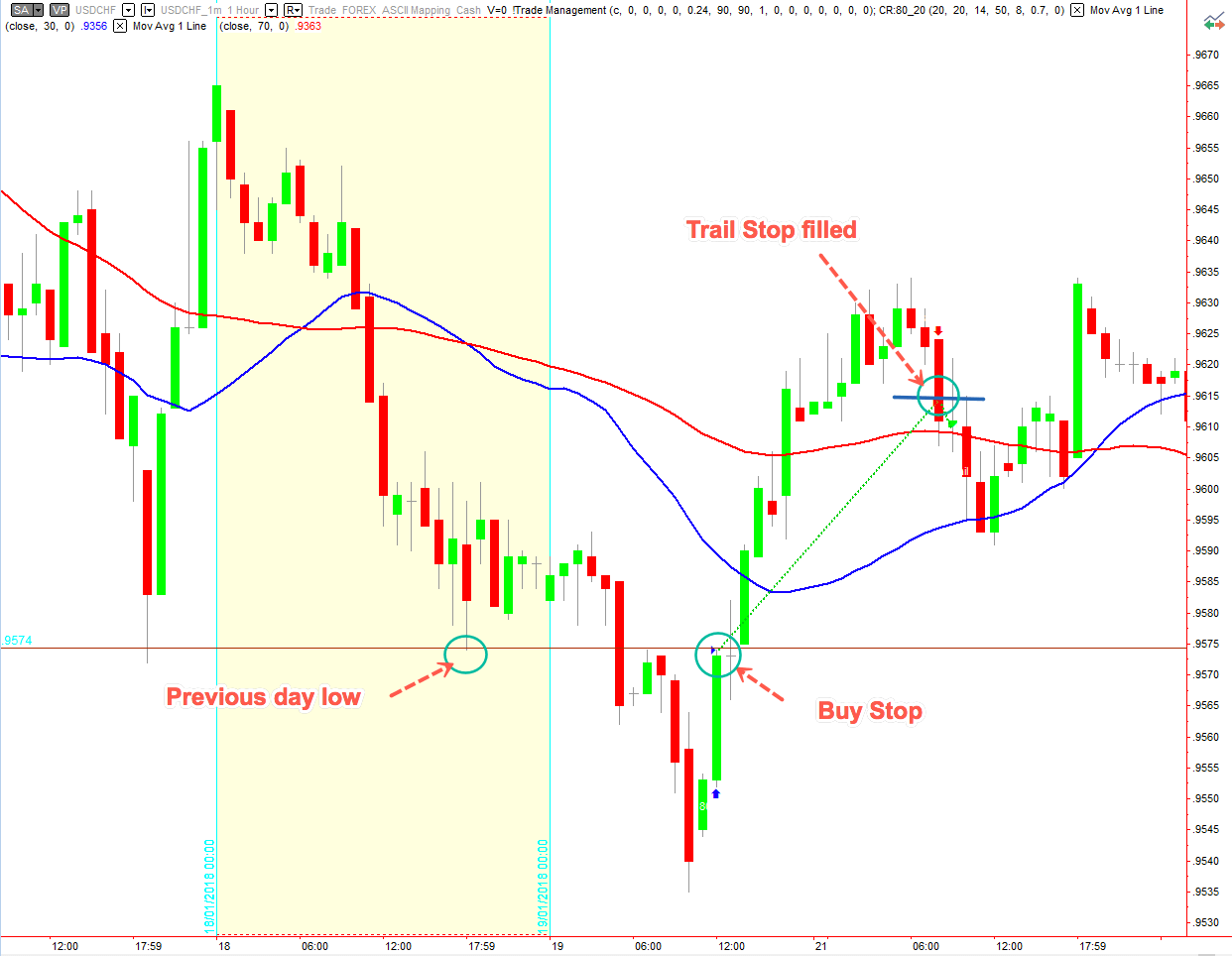
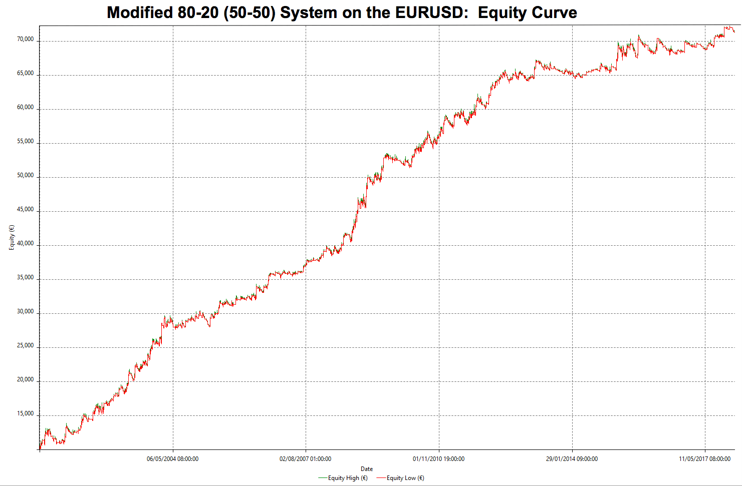
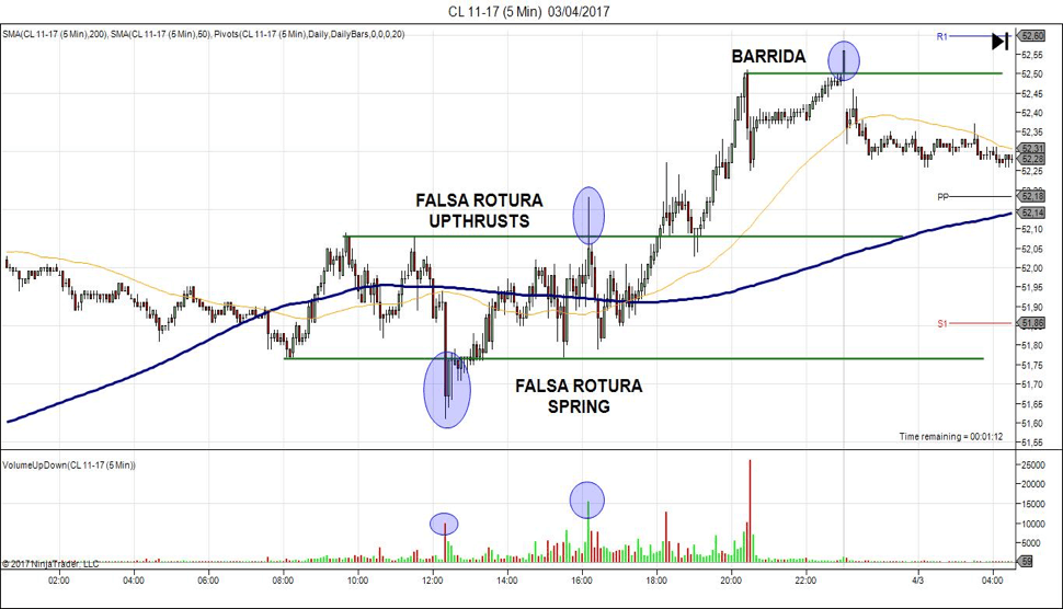
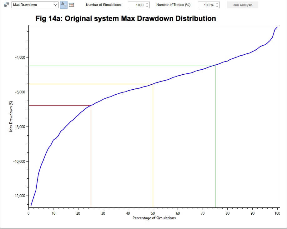
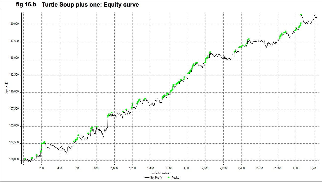
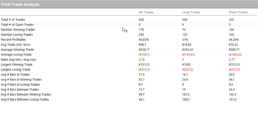
Based on the above results, we set the stop at 0.105% of retraction, and now it looks like this.

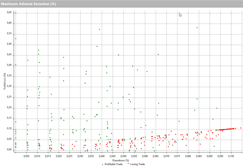
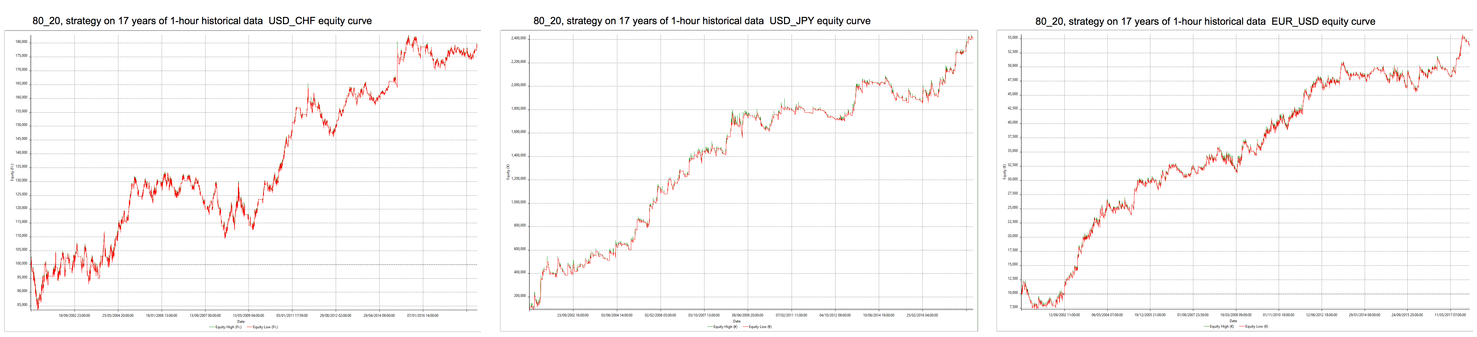
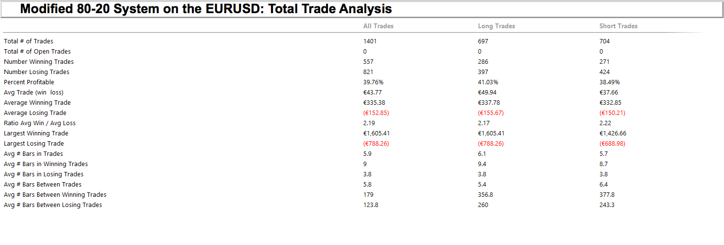
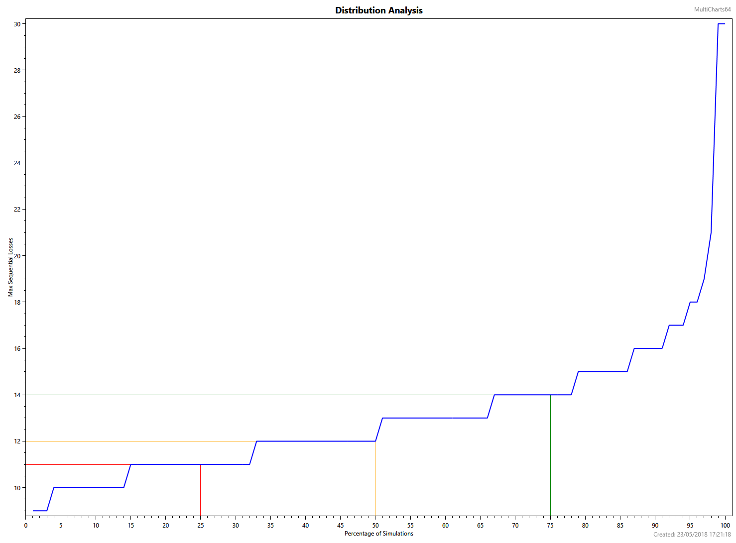
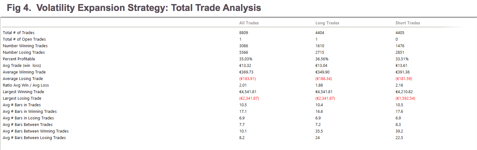
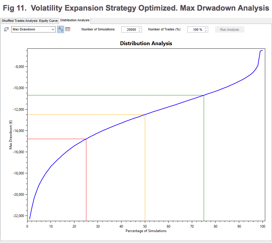
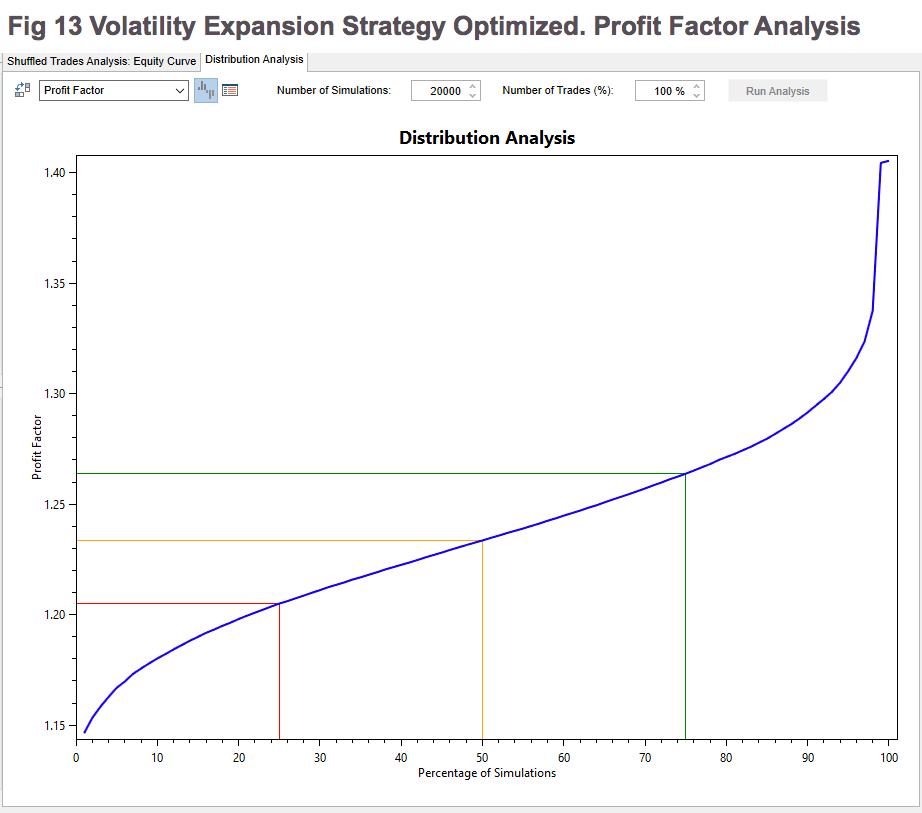
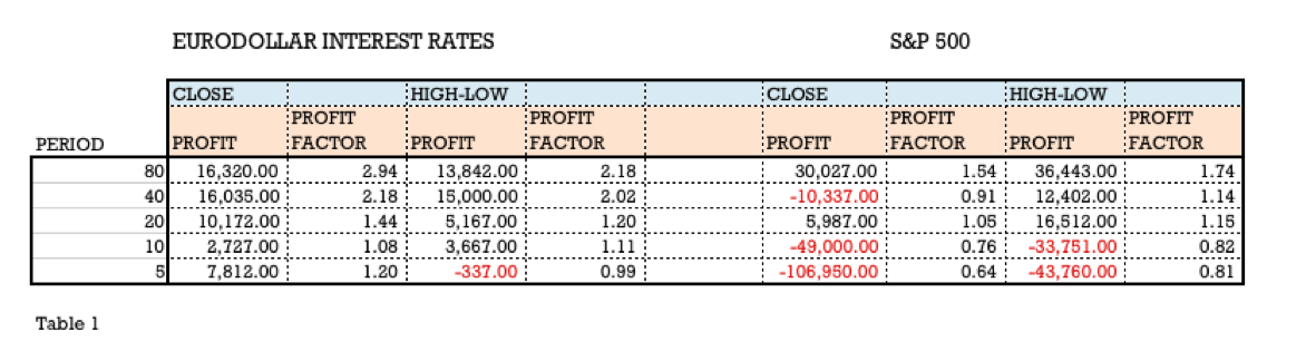
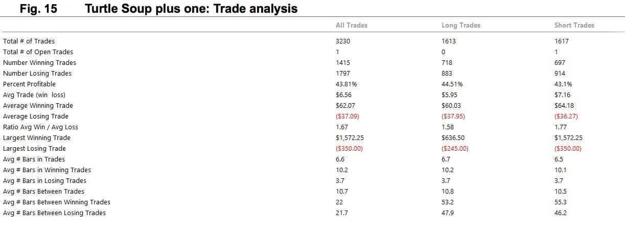
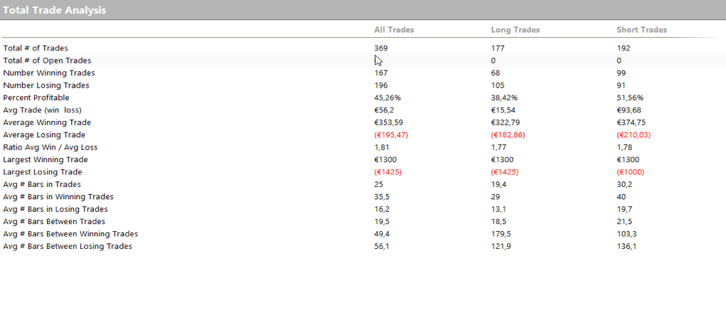
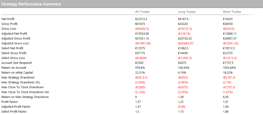
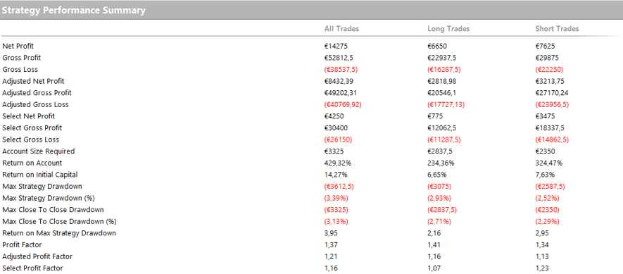
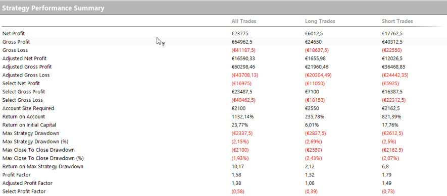
The statistics are as follows:

Statistics have improved. First, the maximum loss has been reduced from -1425 € to -237 € as well as the average loss from -195.47 to -167.24, and the profit-loss ratio has improved from 1.81 to 2.13.

By applying a trailing stop to the system, we can improve some statistical data that will help in the general computation. The use of this type of stop is delicate because it is very easy to be touched by a momentary price retreat. However, its use at a sufficiently loose distance can prevent a trade that is very advanced from becoming lost. In our case, the average loss on the losing trades improve from 167 to 158, and the percentage of winning trades increases slightly in both the long and short sides. It would read as follows:

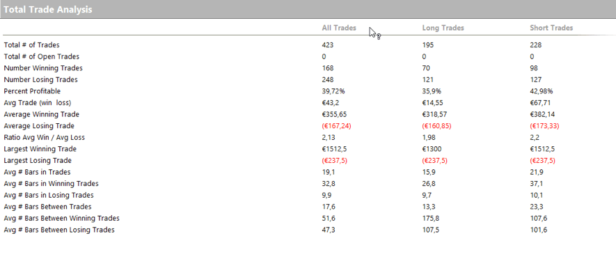
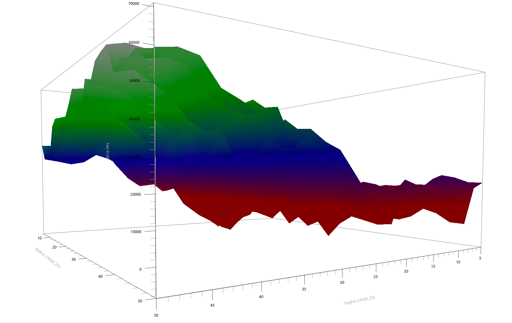
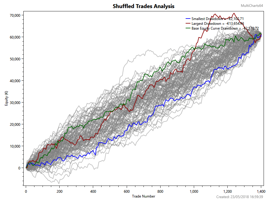
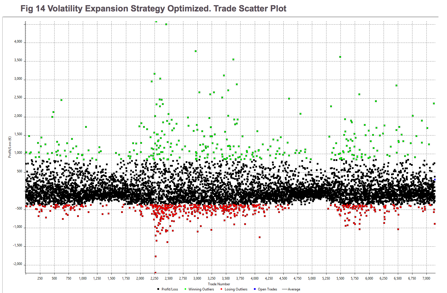
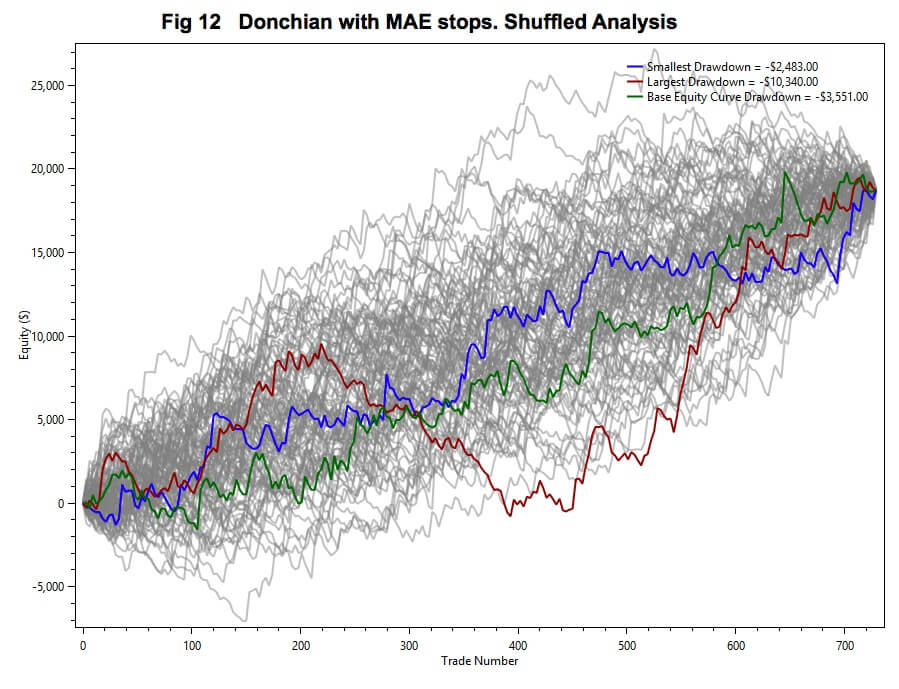
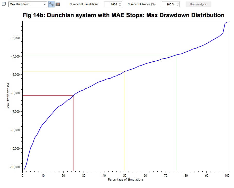
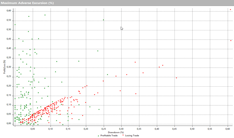
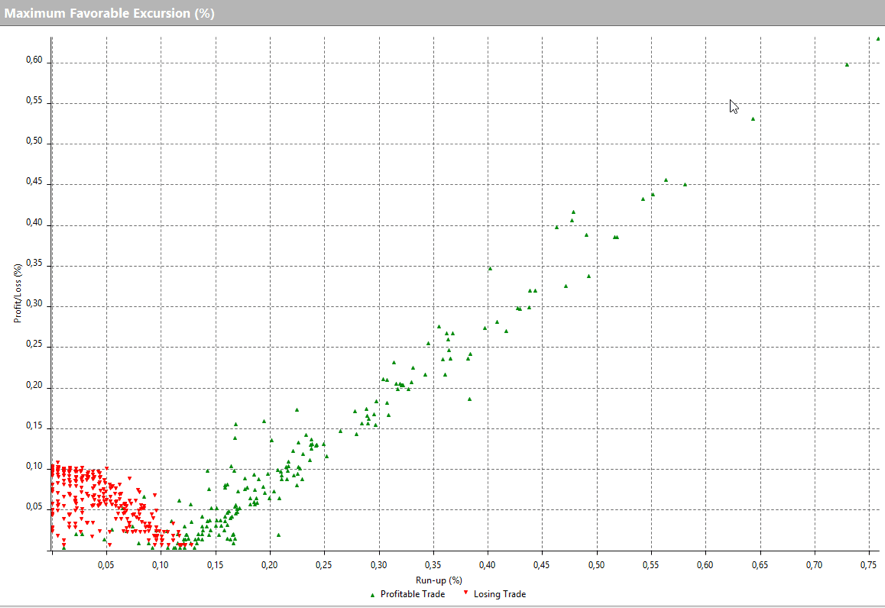
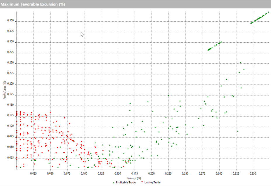
Now to advance the robustness of the system, let’s look at the Maximum Favorable Excursion (MFE) by looking at the following graph.

We see the effect of the Trailing Stop. The trades advance far beyond the point at which they finally close. This is normal using this type of stop. Adjusting them further usually leads to a worsening of the final result of the set.

In the following chart, we see the effect of setting the Trailing Stop 50% closer.

Although it seems better, the total gain is worse, and the drawdown increases.

You can then compare the two options statistics, which leave no doubt.

Statistics with optimal Trailing stop:

Statistics with Trailing stop a 50% more adjusted

Maximum Favorable Excursion

The MFE is found by monitoring the maximum reached during positive operations. Often, we find that our trades end very far from this point. Obviously, our goal must be to get them to stop as close as possible to the MFE. In each particular case, we cannot expect to always close at the absolute maximum. In this case, the methods of traditional technical analysis based on indicators often betray us by getting us out of the market ahead of time or, on the contrary, keeping us while the point of maximum profit goes away.

By searching the MFE, we can detect the most likely area that the winning trades will reach. In this way, we should place our profit target at a point that’s the most probable, statistically speaking. This won’t make our system jump to an absolute possible maximum profit. However, it simplifies the system and makes it more robust by shortening the exposure time to the market.

Finally, a sample of the effect of adding a profit target, taking as reference the MFE. In this case, we separate the behavior of the MFE in the bearish bullish trades since, in the case of indexes and stocks, the market does not usually show symmetry. Experience tells us that there are different characteristics between bull markets and bear markets, although there are authors who question it.

We put a TP (Take Profit) of 27 on bullish and 33 points for the bearish.

What you see is a performance improvement. Although the improvement in net profit does not seem too important, the maximum streak of losses decreases a lot. This procedure reduces the capital necessary for its implementation, and therefore, there is a substantial improvement in percentage profitability. It also increases the net profit and especially the Profit Factor.

Minimum Favorable Excursion

Another concept to evaluate is the Minimum Favorable Excursion. It is to detect the minimum point of advance from which it is unlikely that the price returns on our entrance. This will allow us to move our stops to break even, upon reaching this area and prevent it from ending up in losses.

Conclusion

The statistical method proposed by the MAE and MFE study is revealed as a fully valid system for the study and improvement of any trading system. The use of Maximum Favorable Excursion charts gives us a way to distinguish winning trades from losing trades since they behave differently.

We can see very quickly if there are exploitable behaviors. The behavior of losing trades has its own patterns. It just advances a tiny amount in favor of the entry and then moves against it, and this allows to act consequently by cutting the losses at the right spot where statistically winning trades didn’t reach.

On the other hand, the traditional use of pivots as a reference to locate stops usually leads to losses, since it is the first place where the market seeks liquidity as it minimally weakens a trend.

Finally, the MFE allows us to put the trade into break-even at the right time or even add positions in a favorable environment. It also facilitates the tracking of profit targets. In any case, it is a highly recommended study method to improve automatic or manual systems.

 ©Forex.Academy
Categories
Forex Educational Library

Forex Designing a Trading System (I) – Introduction to Systematic Trading

Trade and money

Trade is a concept that began with the advent of the Homo Sapien, some 20K years back. People, back then, traded their spare hunting pieces for new arrows, spears, or something else he had no time to make himself because he was hunting mammoths.

So, the first questions about what a fair deal was, and, also, how to measure and count things, began.

Trade and agriculture were significant factors that drove the Cro-Magnon men from the caves into civilization.  Everyone started specializing in what they were good at, and people had time to think and test new ideas because they didn’t need to spend time hunting.

Trade brought accounting, the concept of numbers and, finally, mathematics. Ancient account methods were discovered more than 10k years ago by Sumerians in Mesopotamia (the place between two rivers). Also, Babylonians and Egyptians gave value to accounting and measuring the results of their work and trade activities.

Sumerians were the first civilization where agricultural surpluses were big enough that many people could be freed from agricultural work, so, new professions arose, such merchants, home builders, book-keepers, priests, and artists.

The oldest Sumerian writings were records of transactions between buyers and sellers. Money started being used in Mesopotamia as early as 5,000 B.C.  in the form of silver rings. Silver coins were used in Mesopotamia and Egypt as early as 2,600 B.C.

Accounting and money are interlinked. Money was (and still is) the standard way to define the value of products and services, accounting is the method to keep track of earnings, loses and costs and evaluate the use of resources and time.

Currency trading is nothing but a refinement of the concept when several types of currencies are available in an interlinked civilization. Currency trading is the way to search the fair value of currency in relation to other currencies. To traders, accounting is the way to measure the properties and value of their trading system.

Automated versus discretionary

There are several reasons why we’ll need an automated trading system. First of all, people always trade using a system, even when they think they don’t. People trade their beliefs about the market, so their system is their beliefs.

The problem with a system based on just beliefs is that, usually, greed and fear contaminate those beliefs, and, thus, the resulting system behaves like a random system with a handicap against the trader.

Facts

Economic information translates gradually to price changes. Future events aren’t instantly discounted on price.  This is the reason for the existence of trends.

Leverage produces instability in the markets because participants don’t have infinite resources to hold to a losing position. That’s one reason for the cyclic nature of all markets and their fat tail probabilistic density distribution of returns.

There is a segmentation of participants by their risk-taking potential, objectives, and time-frames

The market reacts to new strategies. A new strategy has diminishing returns as it spreads between market participants.

The Market forgets at a long timescale. The success rate of market participants is less than 10%, so there is a high turnover rate. A new generation of traders rarely learn the lessons of the previous generation.

There is no short-term link between price and value.

The market as a noisy structure

All these facts make the markets chaotic, with a fractal-like structure of price paths, a place with millions of traders trading their beliefs, but everyone with a different timeframe and expectations.

This is ok, as no trade is possible if all market participants have the same viewpoint, but the result of hundreds of thousands of beliefs and viewpoints is that the market is as noisy as a random coin flip, as we observe in Fig. 1, reproducing three paths with 200 coin-flip bets, that closely resembles the paths of a currency or futures market.

Contradictory strategies may be both profitable or both losers

On my article about trading using bands, profitable trading VII, I’ve described two totally opposed systems: one was a Donchian breakout system, and the other was The Turtle Soup plus one. Both made money and both traded opposite to each other. That shows that opposing beliefs produce profitable systems.  Trading is not a competition to decide who’s right and who’s wrong. Trading is a business, and the goal of a trading system is to make money, not being right. In fact, none of these two systems were right even 50% of the time, but both were profitable.

Some time ago I developed a mechanical system and was so wrong that I saw almost a continuous downward equity curve. Nice! I thought. This system is so bad that if I switched it from buy to sell and vice-versa it might result in a great system!

Wrong! The reverse system was almost equally bad. That’s the nature of the markets. Nothing is easy or straightforward.

Too much freedom is dangerous

The marketplace is an open environment where a trader can freely choose entry time, direction, the size of her trade and, finally when to exit. No barrier nor rule forces any constraint on a trader. Such freedom to act is the difference between trading and gambling, but it’s a burden to discretionary traders, especially new to this profession because they tend to fall victim to their biases.

The main biases that a novel trader suffers are two: The need to be right and the belief in the law of small numbers. These two biases combined are the main culprits for the trader’s bias to take profits short and let losses run. The need to be right is also the culprit for the trader’s inclination to prefer high-frequency of winners instead of high-expectancy systems. For more on this read my article Trading, a different perspective.

To counteract this unwanted behavior, we’d need to restrict the trader’s freedom by forcing strict entry and exit rules that guarantee a proper discipline and ensure the expected reward to risk, and, at the same time, avoiding emotionally driven trades.

Discretionary versus systematic

The probability of a discretionary trader to succeed is minimal, mainly because, without a set of rules to enter and to exit, the trader immediately fall into the trap of the law of small numbers and starts doubting his system, usually with a substantial loss, as a consequence of considerable leverage.

Most successful traders develop and improve a trading strategy using discipline and objectivity, but this cannot be qualified as a systematic system because its rules are based on their beliefs about the state of the market, their mental state, and other unquantifiable factors.

A systematic trading approach must, conceptually, include:

  • Entry and exit rules should be objective, reproducible, and solely based on their inputs.
  • The strategy must be applied with discipline, without emotional bias.

Basically, a systematic strategy is a model of the behavior of one or several markets. This model defines the decision-making process based on the inputs, without emotional or belief content.

Trading can only be successful using a systematic strategy. If a trader does not follow one, trades will not be executed consistently, and there will be the tendency to second-guess signals, take late entries and premature exits.

Personal adaptation

Developing our own trading system not only gives us confidence in its results, but we’d be able to adapt it to our personal preferences and temperament. We don’t like suits that don’t fit well. A system is like a suit. A perfectly good system for one trader might be impossible to trade for another trader. For instance, a trader might not be comfortable trading on strength while another one cannot trade on weakness. A trader may hate the small losses produced by tight stops, so he favors a system with wide stops. That’s why we need to adapt the system to fit us.

The need to measure and keep records

Measurements allow distinguishing good systems from bad ones. There are several parameters worth measuring, that, later, will be dealt with, but the final objective of measurements is to determine if the trading idea behind the system is worthwhile or useless.

Measurements allow finding where the trading system is weak and optimizing the inadequate parameter to a better value. For instance, we might observe that the system experiences sporadic large losses or that it faces too many whipsaws. Measurements allow searching the sweet spot where stops do its duty to protect our capital while preserving most of the profitable trades.

When the system is already trading live, we might use measurements to adapt it to the current conditions of the market, for example to an increase or decrease of volatility. Measurements help us detect when a system no longer performs as designed, by analyzing the current statistical performance against its original or reference.

Discretionary strategies allow measurements, as well, and, sometimes help to improve a particular parameter, as well, particularly stop-loss position, but, how can this help with entries or exits if they are discretionary or emotionally driven?

Measurements, finally, will help us assess proper risk management and position sizing, based on our objectives and the statistical properties of the developed system. This concept will be developed later on, but my previous article Trading, a different perspective, mentioned above, deals with this theme.

Information

In the discretionary trading style the forex information is categorized into the following areas:

  1. Macroeconomic
  2. Political
  3. Asset-class specific
  4. News driven
  5. Price and volume
  6. Order flow or liquidity driven

In the systematic trading style the information is taken from Price and volume, although lately, some systems are also using sentiment analysis, by scanning the social networks (especially Twitter) and news, with machine learning algorithms. Order flow is left to systems designed for institutional trading because retail forex participants don’t have this information.

In this context, systematic trading simplifies information gathering, by focusing mostly on price and its derivatives: averages and technical studies.

Key Features of a sound system

The essential features a system must accomplish are:

Profitability: The model is profitable in a diversified basket of markets and conditions. To guarantee its profitability over time, we should add another feature: Simplicity. Simple rules tend to be more robust than a large pack of rules. With the later, often, we get extremely good back-tested results but this outcome is the result of overfitting, therefore, future results tend to be dismal.

Quality: the model should show a statistical distribution of returns differentiated from a random system. There are several ways to measure this. The Sharpe Ratio and the Sortino Ratio are two of them. Basically, quality measures a ratio between returns and a measure of the variation of those returns, usually this variation is the standard deviation of returns.

Risk Management and position sizing algorithms: Models are executed using position sizing and risk management algorithms, adapted to the objectives and risk tastes of the trader.

It is desirable that the algorithm for entries and exits be separated from risk management and position sizing.

Sharpe Ratio (SR) and other measures of quality

Sharpe Ratio

Sharpe ratio is a measure of the quality of a system, and is the standard way for the computation of risk-adjusted returns.

SR =ER/ STD(R)

SR = Sharpe ratio

R = Annualized percent returns

ER = Excess returns = R – Risk-free rate

STD = Standard deviation

Sortino Ratio

The Sortino Ratio is a variation of the Sharpe Ratio that seeks to measure only the “bad” volatility. Thus, the divisor is STD(R-) where R- is linked solely to the negative returns. That way the index doesn’t punish possible large positive deviations common in trend following strategies.

Sortino Ratio = ER/SRD(R-)

Coefficient of variation(CV)

The coefficient of variation is the ratio of the standard deviation of the expected returns (E), which is the mean of returns, divided by E. It’s a measure of how smooth is the equity curve. The smaller the value, the smoother the equity curve.

CV = STD(E)/E

SQN

The inverse of CV multiplied by the square root of trades is another measure of the quality of the system. It’s a measure of how good it is in comparison with a random system.

SQ = √N x E/STD(E)

Another, very similar measure of quality comes from Van K. Tharp’s SQN:

SQN = 10*E/STD(E), if the number of samples is more than 100 and

SQN = SQ if the number of samples is less than 100.

The capped SQ value allows comparing performance when the number of trades differs between systems.

Calmar Ratio

CR = R% /Max Drawdown%

It typically measures the ratio over a three year period but can be used on any period, and it’s mental peace index. How stressing the system is, compared to its returns.

CR shrinks as position size grows, so it can be a measure of position oversize if it goes below 5

Defining the parts of the problem

To finally produce a good trading system we need to identify, first, the elements of the problem, and at each one of them find the best solutions available. There are many solutions. There’s no question of right or wrong. The optimal solution is the one that fit us best.

1.    Identify the tradable markets and its features

The forex market is composed of seven major pairs and 16 crosses. The trader should decide about the composition of his trading basket in a way to minimize the correlation of the currently opened trades.

Liquidity is an important factor too. Especially noteworthy is to detect and avoid the hours when liquidity is low, and define a minimum liquidity to accept a trade.

Volatility is also necessary information that needs to be quantified. Too much volatility on a system designed in less volatile conditions may fail miserably. Especial attention to stop placement if they don’t get automatically adjusted based on the current volatility or price ranges.

We should be careful with news-driven volatility. We must decide if we trade that kind of volatility or not, and, if yes, how to fit that into our system.

2.    Identifying the market condition

A trading signal works for a defined market condition. A trend following signal to buy does not work in sideways or down trending markets.

Identify regression to a mean. Usually, mean-reverting conditions happen in short timeframes, due to the spread of trading robots, liquidity availability, and profit taking. Regression to the mean markets merits special entry and exit methods, using some kind of bands or channels, for instance.

Identify oversold and overbought: it is crucial to detect overbought and oversold conditions to avoid trades when it’s too late to get in.

Finally, we must find a way to include all this information in the form of a set-up or trading filter.

3.    The concept and yourself

There are lots of ways to trade a market, but not every one of them will fit all traders. An example of a tough system for myself would be the Donchian breakout system. A robust and simple trend following system, but I know I wouldn’t be comfortable with 35% winners because I know that this means 12% chance of having a streak of 5 losers.

Therefore, to know what fits you, you should try to know yourself and your available time for trading.

Conceptually there are two kinds of players: Those who need frequent small gains and accepts sporadic substantial losses (premium sellers) and those who are willing to pay insurance for disasters, taking periodic small losses in search of large gains (premium buyers).

A premium seeker prefers a hit-and-run style of trading: scalping, mean-reverting, swing trading, support- resistance plays, and similar strategies. A premium seeker has a negatively skewed return distribution, as in Fig. 2:

A premium buyer is a trend follower, an early loss taker, a lottery ticket buyer, a scientist experimenting in search of the cancer cure. He is willing to be wrong several times in a row, looking for the big success: When he finds a trend, he jumps on it with no stops. If proven right, he adds to the position, pyramiding, as soon as new profits allow it. A premium buyer has a positively skewed return distribution, as in Fig. 3:

We notice that the most psychologically pleasing style comes from premium-sellers. The problem with this trading style is that it is not insured for the black-swan-type of risks. He is the risk insurer!

The premium buyer is like a businessperson. A person who is willing to assume the cost of the business for a proper reward. His problem is that he must endure continuous streaks of small loses.

An early loss taker is against the crowd instinct to take profits early, a habit with a negative expectancy, so it pays extra returns to be contrarian.

There is a mixed style where reward to risk is analyzed and optimized. It uses stop protection, while the percentage of winners is enhanced using profit targets.

The main concept for a sound system, in my opinion, is to make sure our distribution of returns has a positive skew. That can be accomplished if we make sure our system has a mean reward-to-risk ratio higher than 1:1, preferably greater than 2:1 but never less than 1:1, and by setting profit targets in tune with the market movements – placing them near resistance or support, and using trail stops.

4.    The law of active management

The Fundamental Law of Active Management was developed by Grinold and Kahn to measure the value of active management, expressed by the information ratio, using only two variables: Manager skill IC and the number of independent investment opportunities N.

IR = IC x √N

If two managers have the same investment skills but one has a more dynamic management, meaning N is higher than the other manager, its return will outperform the less dynamic manager.

This formula can be used in trading strategies, as well:  On two equally smart strategies, the one with more frequent trading will outperform the other. There’s a limitation, though, that this formula doesn’t address: The cost of doing business is more significant the higher the frequency of trading.

5.    Timeframes: Fast vs Slow

The trader’s available daily time has to be considered too. Does the trader have time to be on the screen the whole day or are they busy during work hours, hence, only able to dedicate just a couple of hours at noon to trading.

Unless the trader is willing to use a fully automated system, the time available to them dictates the possible timeframes. A trader who’s busy all day cannot trade signals that show on 1-hour timeframes but is instead forced to focus on swing trading signals that can be analyzed at noon. A full-time trader has all available time-frames at their disposal.

Well summarize here the classification made by Robert Carver on his book Systematic Trading:

·      Very Slow (average holding period: months)

Very slow systems tend to behave like buy and hold portfolios. Trading rules tend to include mean reversion to very long equilibrium such as relative value equity portfolios, that buy on weakness and sell on strength.

As a result of the law of active management, returns from dynamic trading diminish, the lower the trading frequency. Therefore, at large holding periods, the return tends to be poor, unless the skill at timing the market were top notch.

·      Medium (average period hours to days)

The law of active management gives us a clue that this timeframe gets more attractive results than a longer time-frame.

It’s adequate to part-time traders that can do swing trading, working in the evening, searching for signals to be used in hourly and daily charts. From a Forex perspective, these medium-speed timeframes are less crowded with traders. Therefore, strategies may work better than shorter timeframes.

·      Fast( from microseconds to one day)

The Sharpe ratios could be very high in these timeframes, an important portion of the raw returns ought to be spent on costs (commissions and spreads).

6.    Risk

Risk is a broad concept. There are several kinds of risk. The first type of risk is the trade risk. The risk you assume on a particular trade. That’s the monetary distance from entry to your stop loss multiplied by the number of contracts bought or sold.  It’s easy to assess and measure.

The second type of risk is the Potential drawdown a system may experience. This kind of risk is dependent on position size and the percent losers of the system, therefore, we can estimate it with certain accuracy.

Risk can be defined as the variability of results. It’s a statistical value that measures the mean value of the distance between results, and the mean of results and is called standard deviation. The point is that market volatility is shifting and, further, it’s different from asset to asset.

If a trader has a basket of tradable markets, there might happen that one asset is responsible for 60% of the overall volatility on her portfolio, because the position size in that particular asset is higher, compared with others or because its volatility is much higher.

The best way to reduce the overall risk is through diversification and volatility standardization.

Diversification:

To reduce overall risk, there is just one solution: To trade a basket of uncorrelated markets and systems, with risk-adjusted position sizing, so no single market holds a significant portion of the total risk.

Below is the equation of the risk of an n-asset portfolio when there’s no correlation:

𝜎 =√ ( w1 𝜎12 + w2 𝜎22 + … + wn 𝜎n2)

where 𝜎I is the risk on an asset, and wi is the weight of that asset on the basket.

Let’s assume that we hold a basket of equal risk-adjusted positions in 5 uncorrelated markets with a total risk of $10. Therefore, we have a $2 risk exposure on each market, and the correlated total risk would have been 10. But, if the assets were totally uncorrelated, the expected combined risk would be computed using the above equation, then:

Risk =√ (5 x 22) = √20 = 4.47

So, for the same total market exposure, we have lowered our risk by more than half.

Volatility standardisation

Volatility standardization is a powerful idea: It is the adjustment of the position size of different assets, so they have the same expected risk.

This allows having a balanced portfolio where each component has a similar risk. It means, also, that the same trading rule can be applied to different markets if applied with the same standardized risk.

Leverage

The forex industry is attractive for its huge amount of allowed leverage. A trader is allowed to control up to one million euros with a modest 10,000 euro account. That is heaven and hell at the same time. If a trader doesn’t know how to control her risk, he’s surely overtrading.

I recommend reading my small article on position size, but for the sake of clarity, let’s do an exercise.

Let’s compute the maximum dollar risk on a $10,000 account and a maximum tolerable drawdown of 20%, assuming we wanted to withstand 8 consecutive losses.

According to this, we will assume a streak of eight consecutive losses, or 8R.

20% x $10,000 = $2,000 this is our maximum allowed drawdown, and will be distributed over 8 trades, so:

8R = $2,000 = $250, therefore:

Our maximum allowed risk on any trade would be $250 or 2.5% of our running account.

By the way, that value is a bit high. I’d recommend new traders starting with no more than 0.5% risk while beginning with a new system. It’s better to pay less while learning.

The second part of the equation is to compute how many contracts to buy on a particular entry signal.

The risk on one unit is a direct calculation of the difference in points, ticks, pips or cents from entry point to the stop loss multiplied by the minimum allowed lot.


Consider, for example, the risk of a micro-lot of the EUR/USD pair in the following short entry:


Size of a micro-lot: 1,000 units

           Entry point: 1.19344

              Stop loss: 1.19621


We see that the distance from entry to stop loss is 0.00277

Then, the monetary risk for one micro-lot: 0.00277 * 1,000 = € 2.77
Therefore, the proper position size is €250 /€2.77= 90 micro-lots, or 9 mini-lots

Using this concept, we can standardize our position size according to individual risk. For instance, if the unit risk in the previous example were $5 instead, the position size would be:

PS = €250/5 => 50 micro-lots.

That way risk is constant and independent of the distance from entry to stop.

Finally, it’s better to use a percentage of the running capital instead of a fixed euro amount, because, that way, our risk is constantly adapted to our current portfolio size.

7.    The profitability rule

A trading system is profitable over a period if the amount won is higher than the amount lost:

∑Won -∑Lost >0    (1)

The average winning trade is the sum won divided by the number of winning traders Nw.

W =∑Won / N (2)

The average losing trade is then:

L =∑Lost / NL,  (3)  where NL is the number of losing trades.

Thus, equation (1) becomes:

WNwLNL, > 0    (4)

The number of losing trades is the total number of trades minus the winning trades:

NL = N – Nw     (5)

Therefore, substituting (5) and dividing by N, equation (4) becomes:

WNw / N – L(N-Nw) / N > 0     (6)

If we define P = Nw / N,  then (N-Nw) / N = 1-P,  and  (6) becomes:

WP– L(1-P) > 0   ->    W/L x P – (1-P) > 0    (7)

Finally, if we define a Reward to risk ratio as Rwr = W/L  Then we get

P > 1 / (1+ Rwr)     (8)

Equation 8 is the formula that tells the trader the minimum percent winners required on a system to be profitable if its mean reward to risk ratio is Rwr.

Of course, we could solve the problem of the minimum Rwr required on a system with percent winners greater than P.

Rwr  > (1-P)/P     (9)

8.    Parts of a trading system

In upcoming articles, we’ll be discussing all parts of a trading system extensively. Here we are just sketching a skeleton on which to build a successful system.

A trading system is composed of at least of a rule to enter the market and a rule to exit, but it may include the following:

  • A setup rule: A rule defines under which conditions a trade is allowed, for example, a trend following rule.
  • A filter rule: A filter to forbid entries under certain conditions, for example, when there is low volume, or high volatility, the overbought or oversold conditions are reached.
  • An entry rule, defined with price action, moving averages, MACD, Bollinger Bands and so on.
  • A stop-loss, to limit losses in case the trade goes wrong. Optionally a trailing stop.
  • A profit target: Profit target may be monetary, percent, based on supports or resistances, on the touch of a moving average or any other.
  • A position sizing rule. As mentioned before, it should make sure the risk is evenly and correctly set.
  • Optionally, A re-entry rule. The rule decides a re-entry if the stopped trade turns again on the original trade direction.

9.    Chart flow of the development of a trading system

In the next chapters of this series, we will develop on every aspect sketched in this introductory article.


References:

Professional Automated Trading, Eugene A. Durenard

Systematic Trading, Robert Carver

Profitability and Systematic Trading, Michael Harris

Computer Analysis of the Futures Markets, Charles LeBeau, George Lucas

Building Winning Algorithmic Trading Systems, Kevin J. Davey

Categories
Forex Basics

Everything you should master to Detect Trends, and more!

Introduction

In chapter 1, we’ve set the foundations of market classification, what a trend is about, and the dissection of a trend in its several phases. Then we talked about its two dissimilar wave parts: an impulsive wave, followed by a corrective wave.  We dealt with support, resistance, and breakouts. Finally, we talked about channel contractions.

In this second chapter, we’ll learn the methods available in the early discovery of trends: Trendlines, moving averages, and Bollinger band channels.

Trendlines

A trendline is a line drawn touching two or more lows or highs of a bar or candlestick chart. The convention is to draw the line touching the lows if it’s an uptrend and the tops on a downtrend. Sometimes both are drawn to form a channel where the majority of prices fit.

As we see in Fig. 1 the trendline tends to draw resistance levels or supports where the price finds it difficult to cross, bouncing from there, although not always this happens. In Fig. 1 the first trendline has been crossed over by the price, and during the following bars, the slope of the downtrend diminished.  We saw, then, that the first trendline switched its role and now is acting as price support.

When the second trendline was crossed over by the price, a bottom has been created, and a new uptrend started. After a while trending up, we might note that we needed a second trend line to more accurately follow the new bottoms because the uptrend has sped up, and the first trendline is no longer able to track them.

Fig. 2 shows two channels made of trendlines, one descending and the other ascending. The trendline allows us to watch the volatility of the trend and the potential profit within the channel. The trend, as is depicted, has been drawn after it has been developing for a long lapse. Therefore, it’s drawn after the fact.  If we look at the descending channel, we observe that during the middle of the trend, the upper trendline doesn’t touch the price highs. So, this channel would look different at that stage of the chart.

I find more reliable the use of horizontal lines at support and resistance levels and breakouts/breakdowns at the end of a corrective wave. But, if we get a well-behaved trend, such as the second leg in fig 2, a channel might help us assess the channel profitability and assign better targets to our trades. If we use horizontal trendlines together with the trend channel (see Fig 2.b) it’s possible to better visualize profitable entry points and its targets, and, then, compute its reward to risk ratio.  The use of the Williams %R indicator (bottom graph) confirms entry and exit points.

Fig. 2b graph’s horizontal red lines show how resistance becomes the support in the next leg of a trend.

As a summary:

  • A trendline points at the direction of the trend and acts as a support or as a resistance, depending on the price trend direction.
  • If a second trendline is needed, we should pay attention if it shows acceleration or deceleration of the price movement.
  • If the price crosses over or crosses under the trendline, it may show a bottom or a top, and a trend change.
  • A trendline channel helps us assess the potential profitability and assign proper targets to our next trade.

Moving Averages (MA)

Note: At the end of this document, an Appendix discusses some basic statistical definitions, that may help with the formulas presented in this section, although reading it isn’t needed to understand this section.

Some centuries back, Karl Friedrich Gauss demonstrated that an average is the best estimator of random series.

Moving averages are used to smooth the price action. It acts as a low-pass filter, removing most of the fast changes in price, considered as noise. How smooth this pass filter behaves, is defined by its period. A moving average of 3 periods smoothens just three periods, while a 200-period moving average smoothens over the last 200 price values.

Usually, a Moving Average is calculated using the close of every bar, but there can be any other of the price points of a bar, or a weighted average of all price points.

Moving averages are computationally friendly. Thus, it’s easier to build a computerized algorithm using moving average crossovers than using trendlines.

Most Popular types of moving averages

Simple Moving Average(SMA):

The simple moving average is computed as the sum of all prices on the period and divided by the period.

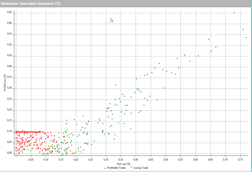
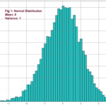
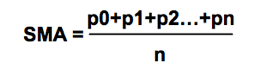
The main issue with the SMA is its sudden change in value if a significant price movement is dropped off, especially if a short period has been chosen.

Average-modified method (AvgOff)

To avoid the drop-off problem of the SMA, the computation of an avgOff MA is made using and average-modified method:

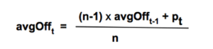
Weighted moving average

The weighted moving average adds a different weight to every price point in the period of calculation before performing the summation. If all weights are 1, then we get the Simple Moving Average.

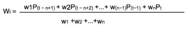
Since we divide by the sum of weights, they don’t need to add up to 1.

A usual form of weight distribution is such that recent prices receive more weight than former prices, so price importance is reduced as it becomes old.

w1 < w2 < w3… < wn

Weights may take any form, most popular being Triangular and exponential weighting.

To implement triangular weighting on a window of n periods, the weights increase linearly from 1 the central element (n/2), then decrease to the last element n.

Exponential weighting is an easy implementation:

EMAt = EMAt-1 + a x (pt Et-1)

Where a, the smoothing constant, is in the interval 0< a < 1

The smoothing property comes at a price:  MA’s lags price, the longer the period, the higher the lag of the average. The use of weighting factors helps reducing it. That’s the reason traders prefer exponential and weighted moving averages: Reducing the lag of the average is thought to improve the edge of entries and exits.

Fig 3 shows how the different flavors of a 30-period MA behave on a chart. We may observe that the front-weighted MA is the one with a slope very close to prices, Exponential MA is faster following price, but Triangular MA is the one with less fake price crosses, along with simple MA: The catch is: We need to test which fits better in our strategy. The experience tells that, sometimes, the simpler, the better.

Detecting the trend using a moving average is simple. We select the average period to be about half the period of the market cycle. Usually, a 30 day/bar MA is adequate for short-term swings.

One method to decide the trend direction is to consider it a bull leg if the bar close is above the moving average; and a bear leg if the close is below the average.

Another method is to watch the slope of the moving average as if it were a trendline. If it bends up, then it’s a bull trend, and if it turns down, it’s a bear trend.

A third method is to use two moving averages:   Fast-Slow (Fast -> smaller period).

In this case, there are two variations:

  1. Moving average crossovers
  2. All the averages are pointing in the same direction.

As with the case of a single MA, a price retracement that touches the slower average is an opportunity to add to the position.

For example, using a 30-10 MA crossover: If the fast MA crosses over the slow MA, we consider it bullish; if it crosses under, bearish.

Using the method of both MA’s pointing in the same direction, we avoid false signals when the fast MA crosses the slow one, but the slow MA keeps pointing up.

When using MA crossovers, we are forbidden to take short trades if the fast MA is above the slow MA, but we’re allowed to add to the position at price pullbacks. Likewise, we’re not allowed to trade on the buy side if the fast MA is below the slow MA.

Using smaller periods, for instance, 5-10 MA, it’s possible to enter and exit the impulsive legs of a trend.  Then, the 10-30MA crossovers are used to allow just one type of trade, depending on the trend direction, and the 5-10 MA crossover is actually used as signal entry and exit (if we don’t use targets). In bull trends, for example, we may enter with the 5MA crossing over the 10MA, and we exit when it crosses under.

Bollinger Band Channel

We already touched channels that were made of two trendlines. There is another computationally friendly channel type that allows early trend detection and trading.

One of my favorite channel types is using Bollinger Bands as a framework to guide me.

A Bollinger Band is a volatility channel and was developed by John Bollinger, which popularized the 20-period, 2 standard deviations (SD) band.

This standard Bollinger band has a centerline that is a simple moving average of the 20-period MA. Then an upper band is drawn that is 2 standard deviations from the mean and a lower band that’s 2 standard deviations below it.

I tend to use two or three 30-period Bollinger bands. The first band is one SD wide, and the second one is two SD apart from the mean. A third band using 3 standard deviations might be, also, useful.

Fig 6 shows a very contracted chart with 3 Bollinger bands to show how it looks and distinguishing periods of low volatility.

During bull trends, the price moves above the mean of the Bollinger band.  During bear markets, the price is below the average line of the bands.

On impulsive legs of a trend, the price goes above 1-SD (or below on downtrends), and it continues moving until it crosses the 2-SD line, sometimes it even crosses the third 3-SD line. Price beyond 2 SDs is a clear sign of overbought or oversold. On corrective legs, the price goes back to the mean. During those phases volatility contracts, and is an excellent place to enter at breakouts or breakdowns of the trading range.

Below Fig. 7 shows an amplified segment of Fig 6, with volatility contractions circled. We may observe, also, how price moves to the mean, after crossing the 2 and 3 std lines.


Grading your performance

According to Dr. Alexander Elder, the market is testing us every day. Only most traders don’t bother looking at their grades.

Channels help us grade the quality of our trades. To do it, you may use two trendlines or some other measure of the channel. If you don’t see one, expand the view of the chart.

When entering a trade, we should measure the height of the channel from the bottom to its top.  Let’s say it’s 100 pips.  Suppose you buy at ¾ of the upper bound and sell 10 pips later. If you take 10 pips out of 100 pips, your trade quality is 10/100 or 1/10. How does this qualify?

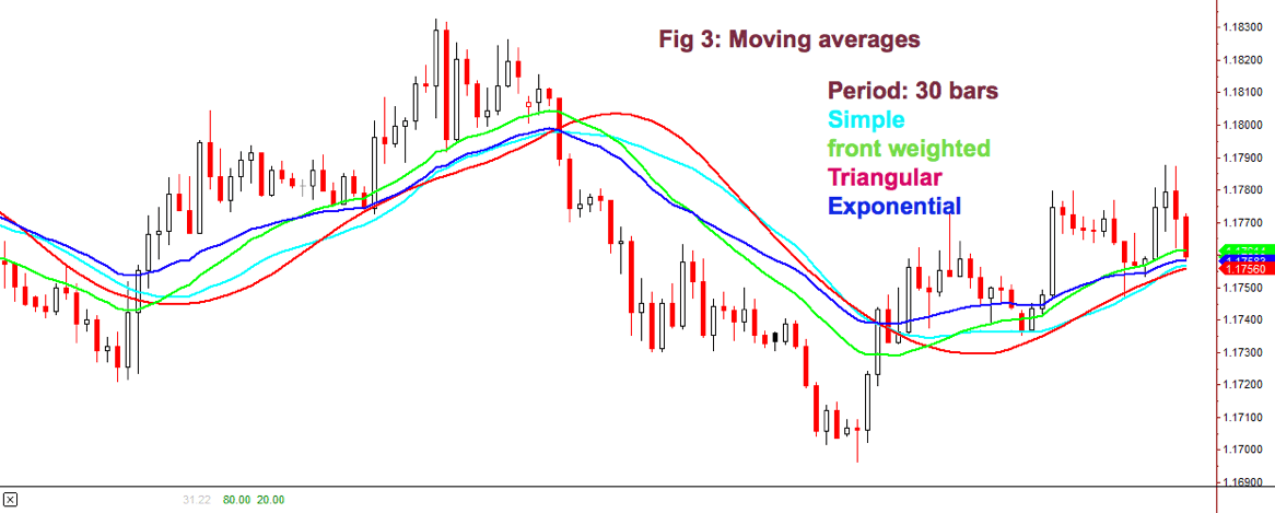
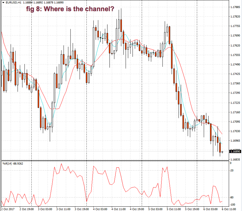
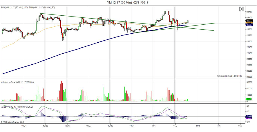
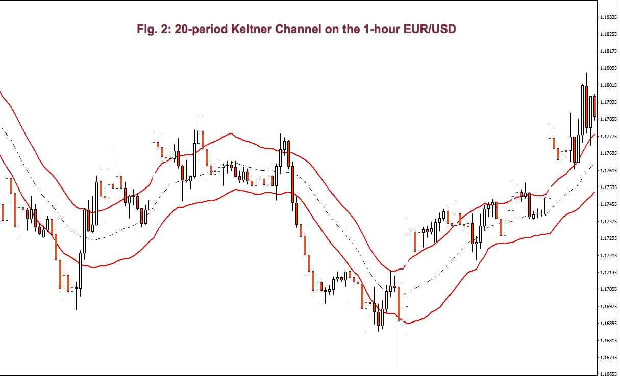
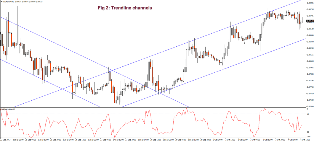
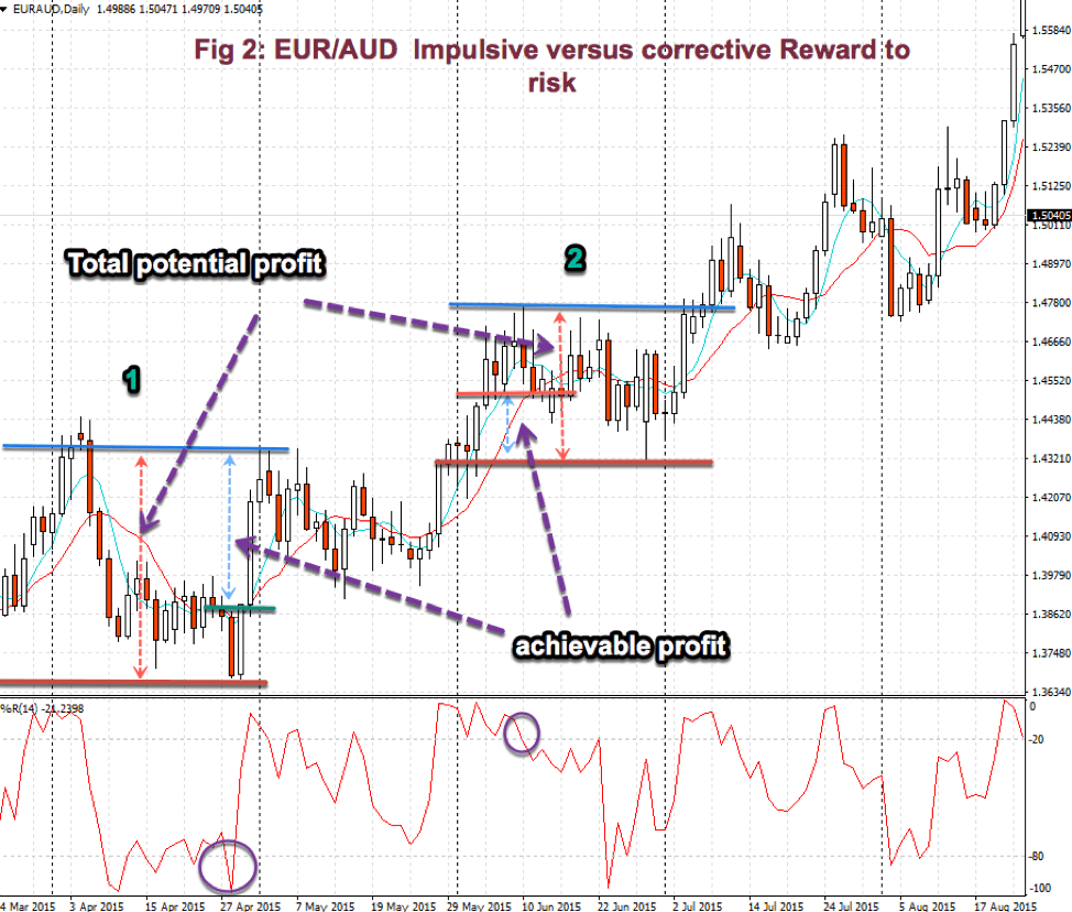
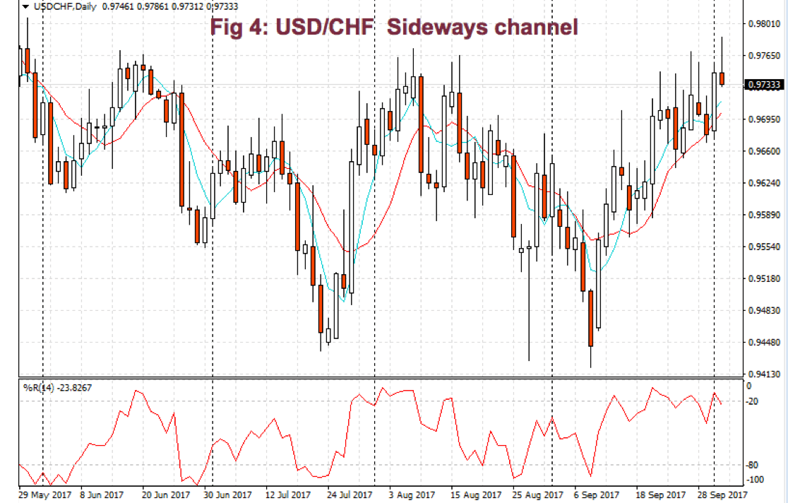
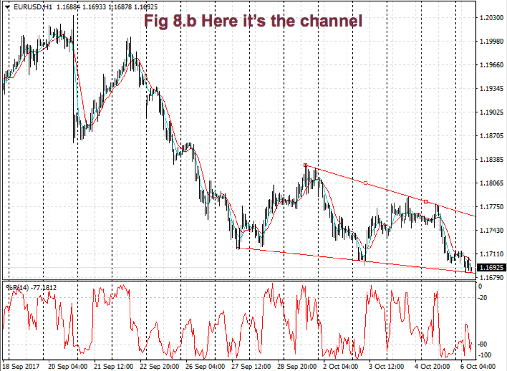
According to Elder’s classification, any trade that takes 30% or more of a channel is credited with an A. If you make between 20 and 30%, your grade will be B. Between 10 and 20% you’re given a C and a D if you make less than 10%.  So, in this case, your grade is C.

Good traders record their performance. Dr. Elder recommends adding a column for the height of the channel and another column for the percentage your trade took out of the channel.

Monitor your trades to see if your performance improves or deteriorated.  Check if it’s steady or erratic.  The information, together with the autopsy of your past trades, helps you spot where are your failures: Entries too late? Are you exiting too soon? Too much time on a losing or an underperforming trade?  A trade against the prevailing trend?


The next chapter will be dedicated to chart patterns.


Appendix: Statistics Overview

Statistics is a branch of mathematics that gives us information about a data set. Usually, the data set cannot be described by an analytical equation because they come from unpredictable or random events. As traders, we need basic knowledge, at least, of statistics for our job.

We can express statistical data numerically and graphically. Abraham de Moivre, back in the XVII century, observed that as the number of events (coin flips) increased, the shape of the binomial distribution approached a very smooth curve. De Moivre thought that if he could find the mathematical formula for this curve, he could solve problems such as the probability of 60 or more heads out of 100 coin flips. This he did, and the curve is called Normal distribution.

This distribution plays a significant role because of the fact that many natural events follow normal distribution shapes.  One of the first applications of this distribution was the error analysis of measurements made in astronomical observations, errors due to imperfect measuring instruments.

The same distribution was also discovered by Laplace in 1778 when he derived the central limit theorem. Laplace showed the central limit theorem holds even when the distribution is not normal and that the larger the sample, the closer its mean would be to the normal distribution.

It was Kark Friedrich Gauss, who derived the actual mathematical formula for the normal distribution. Therefore, now, Normal distribution is also named as Gaussian distribution.

Although prices don’t follow a normal distribution, it’s is used in finance to extract information from prices and trading statistics.

There are two main measures we use routinely: The center of our observations and the variability of the points in our data set from that mean.

There’s one main way to compute the center of a set: the mean. But it’s handy to know also the median if the distribution isn’t symmetrical.

Mean: It’s the average of a set of data. It’s computed adding all the elements of a set and divide by the number of elements:

Mean = Sum(p1-Pn)/n

Median: The median is the value located in the middle of a set after the set has been placed in ascending order. If the set has a symmetrical distribution, the median and the mean are the same or very close to it.

The variability of a data set may be calculated using different methods. Two main ways are used in financial markets:

Range: The easiest way to measure the variability. The range is the difference between the highest and lowest data of a set. On financial data, usually, a variant of the range is calculated: Average true range, which gives the average range over a time interval of the movement of prices.

Sample Variance(Var): Variance is a measure of the mean distance of the data points around its mean. It’s computed by first subtracting the average from all points: (xi-mean) and squaring this value. Then added together and dividing by n-1.

Var = 𝝈2 =∑ (x-mean)2 / (n-1),

whereis the symbol for the sum of all members of the set

By squaring (xi-mean), it takes out the negative sign from points smaller than the mean, so all errors add-up. The division by n-1 instead of n helps us not to be too much optimistic about the error. This measure increments the error measure on small samples, but as the samples increase, its result is closer and closer to a division by n.

If we take the square root of the variance, we obtain the standard deviation (𝝈 – sigma).

 Volatility: Volatility over a time period of a price series is computed by taking the annualized standard deviation of the logarithm of price returns multiplied by the square root of time expressed in days.

𝝈T = 𝝈annually √T


References:

New Systems and Methods 5th edition, Perry Kaufman

Trading with the Odds, Cynthia Kase

Come into my Trading Room, Alexander Elder

History of the Gaussian distribution http://onlinestatbook.com/2/normal_distribution/history_normal.html

https://en.wikipedia.org/wiki/Volatility_(finance)

Further readings:

Profitable Trading – Chapter 1: Market Anatomy

Profitable Trading Chapter III: Chart patterns

Profitable Trading – Computerised Studies I: DMI and ADX

Profitable Trading – Computerized Studies II: MACD

https://www.forex.academy/profitable-trading-computerized-studies-iii-psar/

Profitable Trading (VII) – Computerized Studies: Bands & Envelopes

Profitable Trading VIII – Computerized Studies V: Oscillators

Categories
Forex Educational Library

Profitable Trading – Chapter 1: Market Anatomy

Introduction

In their pursuit of a profitable system or strategy, traders look at past behaviors as a forward indicator of prices.

Indeed, if the price movement is an objective manifestation of the average trader sentiment, then wherever in the future the same sentiment arises, a pattern might take place with a shape similar to the one drawn in the past.  From this belief, it follows that the study of patterns may be of help to find entry and exit points in our pursuit of profits.

There is a catch, though. The human brain is a natural pattern recognizing system. We see patterns everywhere. In ordinary life, that’s the way we recognize things: A round tire, a rectangular table, or a staircase shape. When random events enter into the equation, we continue seeing patterns, although not always, they may exist. Nowadays, Technical Analysis is evolving toward a more evidence-based framework, pushed by authors such as David Aronson, Robert Carver, and others.

I’ll deal with this framework in a future article series, but, throughout the following issues, we’ll deal with the standard TA framework as a foundation for the later. We will develop a base knowledge and the tools to trade the three different market types.

Please keep in mind that, here, we’re dealing with uncertain events, so nothing is 100% sure. Sometimes not even 50% sure. But our objective when trading isn’t being right, but profitable, so as long as our overall performance is positive, the technical signal is good.

Market classification

There are three basic market types:

  • Bull markets: broad ascending trends with sporadic retracements or sideways moves or channels.
  • Bear markets: broad, descending trends with sideways movements or strong and fast bear-trap retracements.

Of course, when trading currency pairs, a bearish market in one pair is a bullish market in its inverse pair, so the tools for bear and bull markets tend to be somewhat similar, and the situations encountered quite symmetric.

Sometimes, lateral markets aren’t perfectly horizontal. The main feature of a lateral market is its increased volatility and noise. The other trait is the seemingly cyclic nature of their movements.

Anatomy of a trend

In Fig 1, we may observe a bullish trend on the EUR/AUD, back in 2015. We may see that prices move in waves. However, the crest of a new wave goes higher than its preceding one. Similarly, its valley is more elevated than preceding valleys, as well.

So, a practical definition of an uptrend is a price pattern with higher highs and higher lows. Consequently, a bearish trend, or downtrend, is, then, a price pattern with lower highs and lower lows.

Trends happen on any time-frame. Even a single bar might be classified as a bull, bear, or lateral. A candlestick with a long white body and short shadows is, in fact, a bullish trend in its tiny time-frame while a long black candle with small shadows accounts as a bearish trend.

Lateral movements on a single bar happen when the candle presents a small body, or none at all, together with long upper and/or lower shadows.

Phases of a bullish trend:

The wavelike pattern, present in most trends, is the result of phases of accumulation, distribution, and sale that draw two different kinds of patterns: One impulsive and one corrective. Every one of these phases accounts as a trend (or lateral channel) in a shorter time frame, which might be composed, at the same time, by shorter trends with its own phases of accumulation, distribution, and selling.

Accumulation phase:

In the later stages of a wave valley, there is accumulation by smart traders who think there is an excellent opportunity with low risk, forming a support level. Sometimes, this support is briefly broken to the downside; stops are taken, and, then, the price back up, again, above support.

After this last trick to fool the weak hands, price starts to climb, slowly at first, faster as momentum grows. In the final moments of this phase, price moves quickly, with substantial price increases on higher volume.

Distribution phase:

In the final stage of an impulsive phase, selling begins by smart profit takers, while the price is still rising, then it reaches overbought levels. A kind of barrier seems to have been established: It’s called a resistance level.

At those levels, more traders are willing to sell than buyers can manage, so price stagnates. Latest bulls don’t have the strength to raise prices beyond that point, but this new leg high is higher than the one in the previous impulsive phase.

Selling phase:

Price moves in a declining channel. Traders that went long at its highs close at a loss. Thus, the price moves down. Then, price recovers as if a new leg up might happen, just to fade again a bit lower than before. Several push-pull phases take place, its pattern like a fading oscillation.

Price reached a new support, and a new accumulation phase begins. Usually, this support is at or near the high of the previous impulse high. This stage draws a corrective pattern.

Phases of a bearish trend

In stock and futures markets, there is a marked asymmetry between bull and bear markets. The former being orderly and, usually, less volatile, except at its beginning, while its ending depicts exuberance and extremely positive expectations. Conversely, bear markets depict much higher volatility, together with fast, bear-trap rallies.

Sell-offs drives prices down much faster than when they are rising. Bear markets tend to be short and fast, losing between 20 to 70% of its value. On stocks, it may lose up to 95% of its value, as it happened to some tech stocks back in 2000 or bank stocks in 2008.

Currency pairs, by its own nature -currency prices moving against each other- make bull and bear phases symmetrical. The discussion above may have been the same if we swap the pair. So A bearish trend in a currency pair has identical stages because it’s just a bullish trend looked from the short side.

What is essential to be aware of is that the impulsive pattern, be it up or down, is the one where we could make more profits with reasonable reward to risk ratios. And the corrective leg (2), the product of a selling phase, is harder to trade and presents more mediocre rewards for its risks.

Fig 2 shows this behavior. We may discover that the Reward to risk channel on the impulsive phase (1) is much broader than on the reactive leg (2) when traded to the short side.

On the impulsive leg, the potential reward is more than 2x its risk, while to the short side, on a corrective phase, it’s less than one, even in the ideal case of taking profits at the lowest low of the channel.

This is a good example of why we should never fight the trend. Instead, we might use a corrective leg to add to a position or entering near support, that is, near the bottom of the channel.

Upside down, this example applies to a bear trend. Here, the impulsive leg, of course, is downward.

There are trends where the channel is more extensive, and both phases, impulsive and corrective, are equally profitable. But those cases are comparable to a sideways market, so the same kind of strategies applies there.

Sideways channels

A sideways channel happens when the price oscillates between two levels that seldom move or move up or down very slowly.  If the channel is wide enough, it may offer trading opportunities, although, usually, volatility is higher, so it’s harder to trade.

Fig 3 shows a sideways channel that took place in the EUR/GBP from Nov. 2016 until Jun. 2017.  Here, we observe there’s a floor level and a ceiling level, where bounces occur.  On this sideways channel, we could split every leg and consider each leg as a bull or bear trend, and go to a shorter time frame to trade it.

But not always, this may be possible. Fig 4 shows the price behavior on the USD/CHF pair for the last five months, from the end of May 2017, till the beginning of October. We may observe that the high volatility that takes place in the last two legs makes it difficult to differentiate impulsive from corrective.  There we must switch to a shorter time frame in search of better behaved impulsive patterns.

A final word about time frames. We should use a higher-order time frame as our guide to decide which side to trade on the shorter frame, then mark support and resistance levels and potential entry points and stops to assess the reward and its risk.

Levels, breakouts, support, and resistance

I’ll tell you here my personal view about levels, support, resistance, and breakouts. People trade their beliefs about the markets. Price is continuously moving in a struggle of two sides, while a third side is watching.

The fight is between those who believe it’ll go up and those thinking it’s already too high and must go down. If the believers on one side are less than on the other hand, price moves against them until a new consensus is made where both parties have similar power.

At price levels where the power of bulls and bears is similar, the price cannot move up or down any longer, until one of the parties weaken or the other gets more strength. In the first case of a price going up and then stagnating, the level is called resistance. The case of a price falling and then stopping its downfall is called support.

On the occasions when the price is pushed beyond resistance, it’s called a breakout. If the price crosses a support level to the downside, it’s called a breakdown. Sometimes the breakout or breakdown is of short duration, price resuming to its previous levels after a few bars. In such cases, it’s called a failed breakout or a failed breakdown. Thus, the passing of time confirms the breakout or breakdown. As time goes, the strength of a support or resistance level increases.

Fig 5 shows a couple of support and resistance channels with two breakouts. Please note that on the second channel, supports are located at the peaks of the sideways channel that preceded the first breakout. This is quite usual, and a persistent pattern in trading charts. Current support levels were, first, resistance levels crossed by a price breakout, becoming supports. Similarly, current resistance levels were support places that were pierced down.

Support and resistance patterns are extraordinarily useful because of their rather good predictive value. Buying at support and selling at resistance is one of the better strategies around, and not only by its success rate but also because they are locations with excellent reward to risk ratio.

Channel contractions

Channel contractions are patterns sometimes called flags and sometimes pennants, wedges, triangles, etc. Although many books about trading patterns make a differentiation between them, they are the same corrective phase, after an impulsive leg.

The critical point to remember about this type of formations is that they are excellent places to trade following the breaking direction. We don’t care which one is it. Usually, it’s a trend continuation, but that doesn’t matter much because the second most important feature of a range contraction is that at those spots, the reward to risk is increased almost double compared to its beginning point.

Fig 6 shows an example of a channel contraction, where we will be able to observe at 1 the risk at its beginning and at 2 the risk at its end. We, also, are able to see that this type of formations is a trend continuation most of the time.

In the next issue, we’ll talk about trendlines, moving averages, and channels.

That’s all for today.

©Forex.Academy


References:

I took some ideas from Essential Technical Analysis, Tools, and Techniques to Spot Market Trends by Leigh Stevens. The rest is mine.

All charts are taken from the MT4 trading platform.