Traders, who operate in the foreign exchange market, read such news every day as: “the consolidation of the dollar led to the fall in the price of gold” or “the price of the euro backed the price of oil”. Although this news is usually published after an event, the relationship between the goods market and the foreign exchange market is felt independently whether we trade in the foreign exchange market or have nothing to do with it.
Theoretically, inflation serves as a correlation between the value of money and the prices of goods, and in this case, the currency does not matter (whether dollars, euros, rubles, British pounds, or Indian rupees). If a week ago the price of gasoline cost 40 rubles per liter and now it is 50 rubles, this means that the ruble in a week was lowered by 25% and the gasoline, on the contrary, increased in price. If gold cost $ 30 per gram in June 2009 and in June 2019 was $ 43, this shows that in 10 years the value of gold in US dollars increased 43% and the dollar, the other way around, fell in price.
Correlation between the goods market and the foreign exchange market. How does it work? They are simple and easy to understand (and also applicable to trading) examples of how money and goods are related and why the correlation between the goods market and the foreign exchange market is a fundamental rule that determines the price of a currency. Let’s try to decipher this theory.
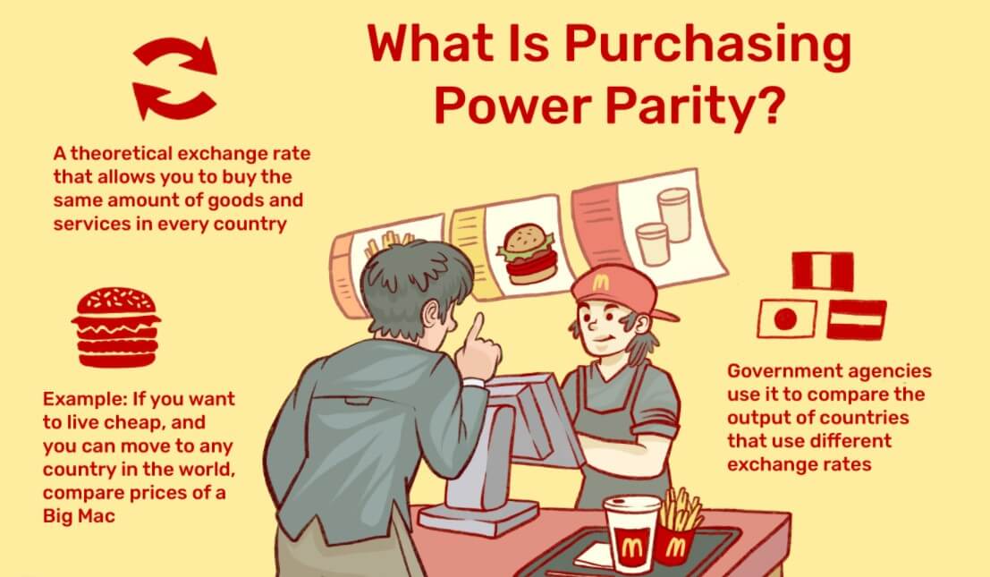
Purchasing Power Parity Theory
Purchasing power parity theory states that the cost of goods in one country should not exceed the cost of goods in another country more than the price of the transport of goods between the two countries. The price of transportation also includes the profit margin of the trader and the change of the standards of one country by the standards of the other. It is also theoretically assumed that there are no artificial trade barriers.
When most of Europe and Asia, back in 1944, were in ruins, a conference was held at the Bretton Woods spa where, for the next twenty-five years, the fate of all the world’s currencies was determined, among which the United States was chosen as the international reference currency. The currencies of other countries were beginning to be traded in dollars, the same dollar was convertible into gold and the troy ounce was worth $ 35. That agreement at that time seemed fair, as the US had 70% of all world reserves and, thanks to the Second World War, it had an international advantage.
The Bretton Woods monetary system existed until 1971 when United States President Richard Nixon unilaterally terminated the agreement, and on 16 March 1973, the treaty is known as the “Jamaica agreement” was signed, which formed the Forex currency market. According to the “Jamaica agreement”, exchange rates would be set in the market on the basis of supply and demand. Since then and to this day the dollar is the main reserve currency, occupies a leading position in the calculation of energy, goods, and gold, and is the main currency used in many financial instruments.
At present, the US dollar position is well described with the word “petrodollar”, and the main volumes of trade in goods, including oil and gold, take place on US exchanges such as NYMEX, COMEX, CME, and ICE. The United States leads in the trade of oil, gold, grains, and many other goods, and the quotations of productive resources are valued in US dollars: gold/dollar (GOLD/$), oil/dollar (WTI/$), corn/dollar (Corn/$), wheat/dollar (Wheat/$), coffee/dollar (Coffee/$), etc.
For the determination of the value of the market of goods or a group of goods there are different indices of raw materials. The best known among them are: Thomson Reuters/CoreCommodity CRB Index (CRY) and Deutsche Bank Commodity Index, which are calculated based on parameters of futures traded on the exchanges indicated above. The exception is for aluminum and nickel prices, which are based on quotations from the London Metal Exchange, calculated in US dollars. Gold prices are also valued in US dollars.
The quotations of foreign currencies are also translated through the value of the dollar: pound/dollar (GBP/USD), euro/dollar (EUR/USD), dollar/ruble (USD/RUB), dollar/franc (USD/CHF), dollar/yen (USD/JPY), etc.
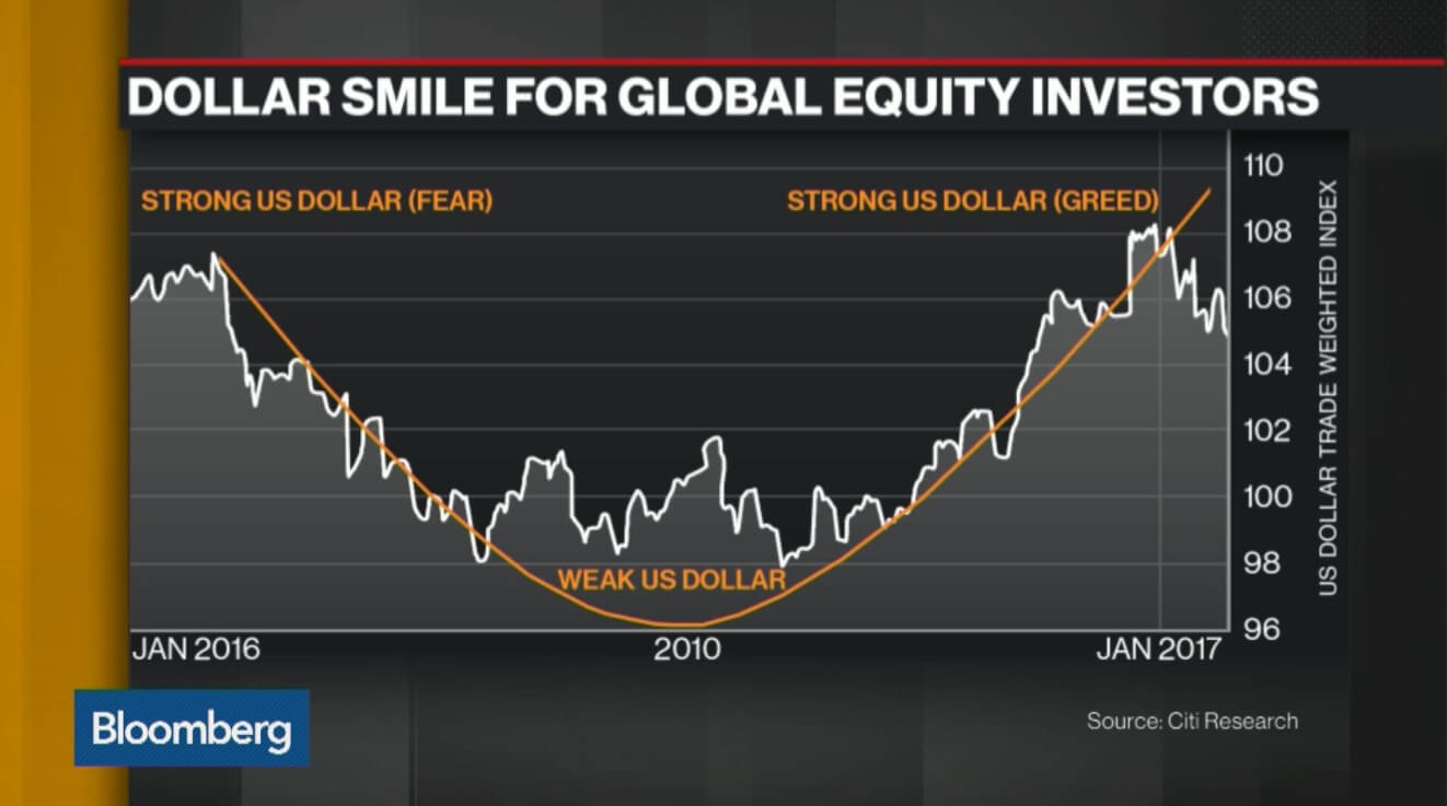
The best known of these is the US dollar index (USDX) measured in relation to the value of a basket of six currencies: the euro (57.6%), the Japanese yen (13.6%), the pound sterling (11.9%), the Canadian dollar (9.1%), the Swiss franc (3.6%) and the Swedish krona (4.2%). The index began in 1971 with a base of 100, and values since then are relative to this base. Therefore, the current rate of index 97 indicates that the exchange rate of the US dollar, relative to the basket of previous currencies, represents 97% of the level of 1971. ¡ A completely insignificant change in 48 years!. But the reality is that it hasn’t always been like this, and in recent years the index has changed considerably from the level of 70 percent in 2009 to the level of 128 percent in 1985.
Do we say “oil,” but do we really mean “dollar”?
As we have already mentioned, the US dollar is used in goods and currencies; the exception is inverse currency pairs, but it is only a mathematical casuistry for the ease of quotation of these currencies. It is very logical to think that at the moment when the dollar rises, the exchange rate of goods decreases, and vice versa, the depreciation of the dollar leads to the rise of currencies and goods markets.
Between July 2014 and July 2017, oil and the dollar correlated with each other with a coefficient of -0.75, that is, they were inversely correlated. Thus, at that time the linear correlation between EUR/USD pair and Brent-type oil in certain periods of time can reach the coefficient of 0.9, that is, it can be very high.
In the preceding paragraph, I purposely emphasized the phrase “in certain periods of time”. The ability to detect periods, in which one or the other factor impacts on quotes, depends on the competition between traders and the level of his training. In this case, there are no clear examples and schemes, everyone has to take this path on their own. But what we do have to warn about is the effects of oil prices on foreign exchange rates increases over time, when the difference in interest rates is small, as in the years 2014-2017, and decreases, when interest rate potential increases, as in the years 2018-2019.
Analysing the correlation between the prices of goods, oil, and the foreign exchange market, it should be noted that the study of the correlation between these assets has a low efficiency. It is better that traders, who ultimately decide to study the issue on their own, focus on monitoring quotes by oscillators, for example, the stochastic indicator or RSI that allows absolute values to be left by the percentage change of some assets compared to others.

We live in the era of hydrocarbons, and oil and its derivatives are the main product whose price affects all other sectors of the economy, which is reflected in the indices. Energy carriers account for 33% of the composition of the Thomson Reuters/CoreCommodity CRB index, regardless of natural gas. As a major part of the Deutsche Bank’s commodity index, petroleum products, and oil amount to 50 percent.
In this way, the change in the price of oil leads to changes in the entire market of goods, from which some dependencies can be deduced: the decline of the dollar leads to the growth of the price of oil and foreign currencies; and vice versa, the rise of the US Dollar contributes to the depreciation of the price of oil and foreign currencies.
It is impossible to predict the beginning and the end of this correlation. For example, the price of the euro may fall, causing the rise of the US dollar, which in turn will contribute to the fall in the price of oil; or if the price of oil begins to rise, the price of the dollar begins to fall, which in turn causes the growth of the euro.
Purchasing Power Parity Assumptions
Purchasing power parity theory takes into account a world in which there is no single reserve currency, assuming many world trade points, which is not in keeping with the current situation. However, the crisis of the world’s dollar-based currency and the trade wars that have been unleashed as a result of Donald Trump’s presidency have forced the governments of major emerging power centers to try to find a gradual replacement of the US dollar as a universal equivalent value.
Thus, for example, in the calculations of Asian goods, the Chinese yuan has already left the Japanese yen behind and is gradually displacing the US dollar from trade. At the St Petersburg Economic Forum in early June, China and Russia agreed to eliminate the US dollar from reciprocal payments and arrangements; Iran and Turkey take the same path.
The tendency to renounce the dollar is barely growing, but it already seems impossible to stop it. The more trade tariffs the US applies, the more the dollar will shift in financial calculations and the faster the US currency will lose its position as the dominant global currency. Trade wars will inevitably lead to the fragmentation of the world economy in several monetary and customs zones, where the theory of purchasing power parity will be in force in a forceful manner, avoiding the intermediate link that is the US dollar. Of course, there is no one who knows for sure when it will happen, but there is no doubt that one day it will happen.
Purchasing power parity theory, like interest rate parity theory, is the fundamental basis of the currency market. In turn, the study of the relationship between the goods market and the foreign exchange market is an important element in the “authentic” fundamental analysis, unlike the studies of different “relevant” economic indicators or informative, which are very often difficult for private traders to analyse due to a lack of their knowledge and resources. However, knowing how it works and thinking nimbly, we will always find a way to apply the basic rules of the currency market to make a profit, even in complicated situations. He who seeks finds!