Categories
Forex Elliott Wave

Impulsive Waves Construction – Part 2

A useful tool for motive wave analysis is the use of channels. In this article, we will review how to use channels to identify motive waves.

Channeling process

A channel is a technical figure that is formed by three points. In Elliott wave theory, channels allow us to identify the potential objective of waves 3 and 5, with “dramatic precision.”

R.N. Elliott, in his work “The Wave Principle” tells us that a channel cannot be drawn if wave two has not ended. Once this wave is complete, we can trace the first channel by connecting a line from the origin of the first impulse to the end of the second wave. Then, a parallel line is projected at the end of the first wave. The following figure shows the process.


Once the third wave is completed, the same process is repeated, this time, we connect the end of wave 1 and 3, and we make the projection at the end of wave 2. This channel will give us an approximation of the end of wave 4. To estimate the end of the fourth wave, we must consider that it should never be more profound than wave 3. The following figure shows this channeling process.


Finally, once the fourth wave is finished, we draw the baseline of the channel linking the ends of waves 2 and 4 and project the parallel line at the end of the third wave. This channel will give us as a possible end of the fifth wave.


The following Silver daily chart shows that the precious metal is completed a sequence of three waves. Currently, the commodity is running in a wave 4 with a potential target at the $17.5 zone.


Categories
Forex Elliott Wave

Impulsive Waves Construction – Part 1

Previously we presented an ideal model of motive waves; however, the real market is not exactly perfect. In this educational article, we will develop the principles of impulsive waves.

The nature of impulsive waves

Before we begin to identify impulsive waves, we must consider the following rules that compose it:

  1. It must have five consecutive segments, or waves, that develop a trend.
  2. Three of these five waves must move in the same direction; this can be bullish or bearish.
  3. After the initial wave, a shorter sequence must be developed in the opposite direction of the first movement. This movement should never be greater than the advance of the first wave.
  4. The third wave must be larger than the second movement.
  5. After the third impulsive movement, a similar sequence to the second wave should be developed. However, the third segment trend must prevail over the fourth.
  6. The fifth wave, in most cases, will be more extense than the fourth movement. If the fifth wave is smaller than the fourth wave, this is called a “failure.”
  7. When comparing the lengths of waves 1, 3, and 5, the third wave does not necessarily have to be the longest. However, it should not be the shortest.

If one of these rules is not followed, then the movement is not an impulse, the structure corresponds to a corrective sequence.

The alternation principle

Elliott defines alternation as a law of nature, as the day and night alternates, the movements of a market also alternate. The alternation principle establishes that when two waves of the same degree are compared, they are different from each other.

We observe the alternation in:

  • The distance that price travels.
  • The duration of each wave.
  • The retracement of the depth of each impulse (waves 2 and 4).
  • The complexity of each wave, that is, the number of internal waves that compose it.

The following daily chart corresponds to the EURAUD cross. In the chart, we observe the alternation in price and time. The first bullish movement began on August 21, 1997, at 1.42014, this wave was developed on 118 days and increased 2,919 pips or 20.55%. Wave 3 surged on 131 days and reported an increase of 19.83% or 3,121.6 pips. Finally, the fifth wave grew in 81 days, advancing 3,059.5 pips, or 17.44%, reaching the high at 2,05983 on October 06, 1998.


In the following EURAUD daily chart, we recognize the alternation in the retracement. From wave 2, we observed that the retrace of wave 1, was developed for 44 days, and the cross plunged 8.05% or 1,377.9 pips. Finally, wave 4 fell 1,334.1 pips (7.07%) of wave 3 in 36 days.


Categories
Forex Elliott Wave

Planning your First Wave Analysis – Part 2

In a previous post, we talked about the ideal structure of an impulsive and corrective wave. Also, we discuss the starting point of the study of a market. In this opportunity, we will deepen the steps to identify a wave.


Watching the waves


Before continuing, we must consider the concept of “wave.” A wave is a defined movement of the market, which is reflected in a price variation. Depending on the price action, the change may have a higher or slower speed, but it will never be perfectly horizontal or vertical.

Depending on the sequence of a group of waves, the market may develop an impulsive or a corrective wave structure. An “impulsive wave” is made up of five waves with a relationship of the same degree. On the other hand, a “corrective wave” is composed of a set of three waves. The following figure shows an ideal impulsive and corrective wave.


Wave proportionality

Once we define the start point and the timeframe of the market study, we must consider that waves should have specified “proportionality.” Consider that some Elliott structures could not be easily visible by simple observation. For this reason, we must be flexible in terms of the selection of the timeframe to analyze. Remember that the same timeframe will not necessarily useful to examine all markets. Elliott, in his “Treatise,” reminds us that in markets with low volatility, the weekly chart may be more fit than the daily chart.


Price and time relationship

In a sequential movement, the price action is developed following the relation between price and time. On the following chart, we observe the Financial Select Index ETF (AMEX: XLF) on a weekly timeframe. In the example, we note that the sequence starts in the March 2009 low at $ 4.47, and ends when XLF reached the February 2011 high at $ 13.90. After this top, XLF developed a retrace in February 2011, which led to a higher low at $ 10.02.


In this example, there is a similarity in the advance and retracement of the price with the time. In summary, the movement of two consecutive waves of the same degree cannot be less than one-third (1/3) of the greater in terms of price and time.

Categories
Forex Elliott Wave

Planning the First Wave Analysis – Part 1

Before to start to analyze any market, it’s necessary to set-up the chart earlier to begin to identify motive and corrective waves. In this article, we will learn how to start to analyze the market applying the Elliott Wave Theory.


Setting-up the first chart

The first step consists of choosing the market to be studied, and then select a starting point for the analysis. Once we decided the market of interest and the inception point, in a monthly chart, we will identify the highs and lows of the asset in the order of appearance. After that, we must establish the relevant date and price of every segment.

As an example, the following chart corresponds to the DAX futures in a monthly timeframe. As you can notice, there are identified the “relevant” highs and lows from March 2000 until the present.

Once we defined the starting point,  we will begin the analysis by moving our timeframe from higher to lower. In means, from monthly to daily timeframe, and even to an hourly chart. However, this could demand you extra time to update the analysis.

The identification process

When the identification is complete, we must distinguish the start and end of each wave. From our example, we will start from the March 2009 low at 3,588.5 pts, until the January 2019 high at 13,181.5 pts.

The same process must be realized in the weekly and daily timeframe. As you can notice, we still do not begin to talk about motive and corrective waves. The reason is that the first step is to learn to recognize the movement under study.

As was discussed in the previous article, we will use labels to identify each wave. In our example of the FDAX monthly chart is as follows.


Summarizing, the monthly chart of the FDAX shows a bullish sequence which currently should be developing a wave ((5)). As we learned, waves ((1)), ((3)), and ((5)) moves in the bullish trend direction; it is a motive wave. The waves ((2)), and ((4)) retraces the main trend movement, or in other words, these waves are corrective of the principal trend.

Categories
Forex Elliott Wave

Fundamentals of Elliott Wave Theory – Part 3

Until now, we have defined two kinds of waves, motive and corrective. In this article, we will introduce the concept of “degree,” which will help us in the process of waves identification.

The concept of degree

Elliott defined a series of “degrees” to maintain a hierarchical waves order. This order is based mainly on the relationship that the wave develops over time. In other words, while higher is the time elapsed in the wave formation, greater will be the wave degree.

The term “degree” must be considered in relative terms about the price and time relationship. It should not be considered strictly according to the duration, for example, a day, a week, or a month.

The blue box shows a bullish impulsive wave developed over126 days which attained a 25.95% advance. This wave started from the low of December 26, 2018, when the price found support at 2,346.6 pts and ended on May 1, 2019, when it hit the top at 2,954.4 pts. If we remember the basic structure of a wave, we can see that the upward movement was developed in five waves.

In the red box, we observe a corrective wave sequence disclosed in three waves. This retracement began on May 1 and ended on June 3, 2019, when SPX plunged to 2,728.8 pts. The bearish move unfolded over 33 days and eased 7.67%.


R.N. Elliott, in his work “The Wave Principle” defined a series of degrees, with specific terminology and it’s as follows:

  • Grand Super Cycle.
  • Super Cycle.
  • Cycle.
  • Primary.
  • Intermediate.
  • Minor.
  • Minute.
  • Minuette.
  • Sub-Minuette.

However, Prechter & Frost, in “Elliott Wave Principle” added six degrees:

  • Supermillennium.
  • Millennium.
  • Submillennium.
  • Micro.
  • Submicro.
  • Miniscule.

Despite the wide-spread degrees, Hamilton Bolton says that the most common degrees used are Minor, Intermediate, and Primary.

Wave Labeling

Labels are useful to keep the order in the wave analysis. It’s necessary to assign a symbol on each wave of each wave that is studied. In the Elliott Wave Theory there is a set of labels for each degree as follows:

The wave labels are essential to understand the current market position and will allow us to respond to the question “where goes the market?”.

The following chart corresponds to the application of waves labeling. In this case, the SPX daily chart developed a complete cycle of Intermediate degree.


Categories
Forex Elliott Wave

Fundamentals of Elliott Wave Theory – Part 2

Waves develop in two classes, impulses and corrections. Impulsive movements are characterized by having a five-wave structure. Corrective waves, on the other hand, growth creating a three-wave structure. In this article, we will introduce the concept of motive waves, corrective waves, and cycles.

Motive waves

Motive waves receive this denomination because they create movement, or “impulse” to the price action, as it follows a trend. In the following figure examining the case of a bull market, waves 1, 3 and 5, are impulsive waves. This structure is analogous for a bear market.


Corrective waves

Corrective waves, as the name implies, are characterized by pushing back the price of the dominant trend. From the previous figure, waves 2 and 4 correspond to the corrective waves.

Cycle concept

As we have seen previously, a wave is composed of five waves, and a complete cycle is composed of eight waves, an impulsive part and a corrective part. For convenience in the identification process, we will label motive waves with numbers and corrective waves with letters. Later we will see the usefulness of wave identification to understand the stage in which the market under study is.


When an eight-wave cycle is completed, a new cycle of the same degree begins, as shown in the following figure. This formation generates a five waves sequence of a higher degree. At the moment, you should not be worried about the identification symbols. Elliott defined the labels and should be understood as a tool to help in the study, and not an objective in itself.


Recognizing this structure is essential to understanding the nature of the wave theory.

Categories
Forex Elliott Wave

Fundamentals of Elliott Wave Theory – Part 1

Ralph Nelson Elliott developed the Wave Theory in the 1930s. Elliott discovered that prices followed a sequence of repetitive patterns in form, but not in time and amplitude. He called these patterns “waves,” he also recognized that each movement was composed of five waves.

The Elliott Wave Theory is not a trading system nor a forecasting tool, but, rather, a description of market behavior. In this sense, Elliott waves enable us to understand the current price position and the scenarios that can be anticipated from it. In our first Elliott’s wave theory article, we will review its history and its underlying principles.

Nature and waves

In 1934, R.N. Elliott published his work “The Wave Principle.” It is this treatise, as he calls it, explains the basics of wave theory. In this work, Elliott explains that everything in nature is governed by a law which its causes could be unknown. However, when the law is known, forecasts can be made, regardless of whether or not the reasons that originated it are known. Both nature and universe, some phenomena are repetitive and can be predicted; for example, the lunar phases, the year seasons, the tides, and so on.

Human interactions are part of nature and are no exception in wave theory. The most common socio-economic activity is realized in the financial markets. Elliott remembers us that “there is no socio-economic activity in which so many resources have been allocated and with neither successful results as financial markets.” In this context, wave theory allows us to have an understanding of the current state of financial markets and their possible next path.

The five-wave structure

According to R.N. Elliott, the financial markets as a socio-economic activity hold a specific structure composed of five waves. These waves move in the direction of the dominant trend and are identified as wave 1, 3, and 5. Similarly, as the market is moving forward, an opposite movement is identified as wave 2 and wave 4. These movements happen against the primary trend.

Elliott, facing the question of why five waves and not another number, in his treatise explains that “it is a secret of nature” and it is not his goal to determine the origin or explanation of the five movements.

Elliott observed that wave 2 never moves beyond the beginning of wave 1, wave 3 is never the shortest, and wave 4 never enters the territory of wave 1. The following figure shows the basic structure of a five waves sequence.


Categories
Forex Trading Strategies

STRATEGY 6: Elliot waves

Foreword

All our strategies are based on input setups that have a prior market reading context, which is equal to, or more important than the pattern itself. We recommend learning with Forex Academy traders to contextualize the market, so we always know what situation we are in.

With this being said, we are going to see what this strategy consists of and how we apply it to the market.

The Elliott Wave Theory

Elliot wave theory offers us different investment opportunities both in favor of the trend and against it. Elliott identified a particular structure to price movements in the financial markets, a basic 5-wave impulse sequence (three impulses and two correctives) and 3-wave corrective sequence.

Let’s see an example for a better understanding of this theory (click on the image to enlarge):


The chart above shows a rising 5-wave sequence. Waves 1, 3, and 5 are impulse waves because they move with the trend. Waves 2 and 4 are corrective waves because they move against this bigger trend. A basic impulse advance forms a 5-wave sequence.

The trend is followed by a corrective phase, also known as ABC correction. Notice that waves A and C are impulse waves. Wave B, on the other hand, moves against the larger degree wave and is a corrective wave.

By combining a basic 5-wave impulse sequence with a basic 3-wave corrective sequence, a complete Elliott Wave sequence has been generated, with a total of 8 waves. According to Elliott, this whole sequence is divided into two distinct phases: the impulse phase and the corrective phase. The ABC corrective phase represents a correction of the larger impulse phase.

The Elliott Wave is fractal. This means that the wave structure for one big cycle (Super Cycle) is the same as for one minute. So we will be able to work in any timeframe.

Let’s see the three rules for our trading:

  • Key 1: Wave 2 cannot retrace more than 100% of Wave 1.
  • Key 2: Wave 3 can never be the shortest of the three impulse waves.
  • Key 3: Wave 4 can never overlap Wave 1.
  • We could trade in favor of the trend on wave 3 and wave  5  and only against the trend once wave 5  has finished.

To know when a wave may have finished, we can use Fibonacci projections and retracement. Fibonacci ratios 38.2%, 50.0%, and 61.8% for retracements and 161.8%, 261.8% and 461.8% for Price Projections and Extensions.

© Forex.Academy

Categories
Forex Educational Library

Trading using The Elliott Wave III: Applying Fibonacci Ratios and the Square Root of Two to Elliott Waves


Background

Traders use the Elliott Wave mostly as a continuously developing price map, on which they try to guess the most probable future path. Sometimes the trader waits for some unfinished wave to end, to pull the trigger or take profits. When this occurs, he or she commonly uses Fibonacci ratios in trading to forecast a price level for that event.

Ian Copsey on his book The Case for Modification of R.N. Elliott’s Impulsive Wave Structure, says he has found that harmonic ratios derived from the square root of two are also a very helpful tool.

My personal belief is that those ratios are really artefacts, a product of the random nature of the trading activity. In the age of computers and Big Data, a statistical study on the retracements ratios might reveal much more precise information about those proportions. Even better, a computer study might be developed to show the most likely retracement levels as a function of the latest N-retracements, taking account of the recent volatility changes.

Nonetheless, Fibonacci ratios and Sqrt-2 ratios may serve as an approximation to forecast retracements or extensions when a better information tool is unavailable.

Fibonacci

Leonardo Pisano Bigollo (1170-1250), known as Leonardo Fibonacci, was an Italian mathematician and traveller, who studied and brought the Indo-Arabic numerical system to Europe. This revolutionary numerical system on which the absolute value of a digit is established by its position within the number made possible the mathematical and scientific revolution in Europe.

In his Liber Abaci book of 1202, Fibonacci introduced the arithmetic systems he learned from the merchants working on the Mediterranean coast that he called modus Indorum (The way of the Indians). The book made a case for a 0-9 digits and place value, as well as examples of how to use it in business to calculate interest rates, money-changing, and other applications.

The Fibonacci sequence

The book also discusses irrational numbers,  prime numbers, and the Fibonacci series, as a solution to the problem of the growth of a population of rabbits.

The Fibonacci sequence starts with two ones: 1,1. The following numbers in the series are calculated as the sum of the preceding two numbers. He carried the calculation up to 377, but he didn’t discuss the golden ratio as the limit ratio of consecutive numbers in the sequence.

Below, Table 1 shows in yellow the first 27 Fibonacci numbers. The other columns, from 1 to 6 show the results of the n-following divisions, as a percentage. That is the result of dividing the Fibonacci number by next one, two apart, three apart etc.

Fibonacci ratios in trading

The last column shows the stabilized Fibonacci ratios generated:

elliott wave fibonacci ratios


Table 2 shows the Fibonacci ratios of the n-preceding division as a percentage.

FIBONACCI RATIOS N PRECEDING

As with the preceding table, the last column shows the stabilized Fibonacci ratios generated:

Fibonacci ratios generated

Two more sets of Fibonacci multiplying ratios are obtained by multiplication and division of the N-following ratios:

FIBONACCI MULTIPLYING RATIOS


FIBONACCI DIVIDING RATIOS

As we can observe, except for ratios smaller than 5% and the 100% ratio, all of them are already present in the original series.

The Square root of two

Well, the square root of two is the first known irrational number, and the one that raised heated passions in ancient Greece, that ended with a crime. At a date around 520 BC, a man called Hippasus of Metapontum was dropped from a boat into open waters to die.  The man’s crime was revealing to the world a “dirty” mathematical secret. The secret of the relation between the sides of the square triangle of length 1, and its hypotenuse.

According to the well known Pythagoras theorem, the sum of the squares of the sides a rectangle is equal to the hypotenuse squared.

Therefore, for unity sides: 12+12 = 2, therefore the hypotenuse length is the square root of 2.

Pythagoras Theorem - Forex Academy

The square root of two including its four decimal places is 1.4242

This article is not focused on the proof that the square root of two is not rational, so I’d recommend the curious reader the following page:

https://divisbyzero.com/2009/10/06/tennenbaums-proof-of-the-irrationality-of-the-square-root-of-2/

Ian Copsey explains that he was told about this ratio applied to the markets by some acquaintance, who stated that it was commonly occurring between musical notes.

After studying it, Mr Copsey began to find out that two derivations of this ratio usually happened: 41.4% and it complementary 58.6%, being 100-41.4%.

Usual wave relationships

Ian Copsey says in his book that, after many research hours into normal relationships between waves, he has found the most usual to be:

Fibonacci: 5.6%, 9%, 14.6%, 23.6%, 33.3%, 38.2%, 50%, 61.8%, 66.6%, 76.4%, 85.4%, 91%, and 94.4%

To this list, you can add those derived from the square root of 2: 41.4% and 58.6%.

And, specifically on Wave (iii), it’s possible to take those ratios and add 100%, 200% and on occasions 300% and 400%.

The most common extensions he has found were: 138.2%, 176.4%, 223.6%, 261.8%, 276.4%, and 285.4%. Additionally, but less frequently, he found 158.6%, 166.7%, 238.2%, and 361.8% and occasionally 423.6% and also 461.8%

It’s important to observe the underlying ratios of a particular market trend. It’s better to stick with the ratios that often show in the most recent retracements of the same kind.

As is usual, the help of visual channels, spotting important supports and resistances or pivot points may show which one of those ratios best fit the rest of the clues.

It is also noteworthy that the projections of the Wave (v) and also of the Wave (c) should match the end of higher-order waves as well, so the most probable final ratio is the result of that confluence.

The data below was taken from Mr Copsey’s study, published in the referred book.

Wave (i)

There is no relationship to any previous wave as this is the start of a five-wave sequence.

Wave (ii)

This is a corrective wave of Wave (i). This retracement is one of the most difficult to assess. According to Ian Copsey, it can go from 14.5% up to 100%. He also mentions that on a 5 min chart it’s complicated to observe the sub-waves composing Wave(ii), however on a daily chart it shows the typical A-B-C pattern or, even, more complex patterns.

Wave (iii)

Wave (iii) is an extension of Wave (i), projected from the end of wave (ii).

Projections:

  • The most typical forecast are 176.4%, 185.4%, 190.02%, 223.6%, 276.4%, and 285.4% projections of Wave (i).
  • Less recurring projections are: 138.2%, 166.7%%, and 261.8%.
  • Sporadically it goes to: 123.6%, 238.2%, 361.8%, 423.6%, and 476.4%.

Wave (iv)

Wave (iv) is, of course, a retracement starting from the top of Wave (iii). At this stage, noting the implications of the alternation rule with Wave (ii) or Wave (b) there is a stronger basis to identify the end of the pullback.

Potential retracement percentages:

  • For small retracements: 14.6%, 23.6%, 33.3%, and 38.2%.
  • For mid retracements: 41.4% and 50%.
  • For intense retracements: 58.6% and less often 61.8% or 66.7%.

Wave (v)

Wave (v) is an extension of the total price move from the beginning of Wave (i) to the end of Wave (iii), projected from the end of Wave (iv).

Having identified Wave (iv) makes it much easier to build up a projection for Wave (v).

Projections:

  • The bulk of projections go to 61.8%, 66.7%, and 76.4%.
  • In a truncated Wave (v), usual ratios are 58.6% and 50%.
  • In an extended Wave (v), the most usual projections are: 85.6%, 100%, 114.4%, and sometimes 123.6% and 138.2%.

Wave (A)

Wave (A) is similar to Wave (I) in its unpredictability. There is no reference to spot its end because there is no relation to other prior waves. The best method is to find a higher order price channel in which this wave might end, observe support/resistance levels or pivot points.

Another method is to go to a shorter time frame, watch the 5-wave pattern that constitutes the A wave and try to project Wave (v) by matching it with a previous Wave (B) of Wave (v) or the prior Wave (iv).

Wave (B)

Wave (B) is a retracement of Wave (A), but it’s a correction within a correction so that it can be really complicated and random. The retracement ratios range from 15% to 100%. The use of pivot, swing high and low, and support/resistance levels give more clues than simple mathematical ratios.

As stated in other articles, it doesn’t pay to trade Wave (B) or any other 3-wave corrective pattern for that matter, because of it’s poor reward-to-risk ratio.

Wave (C)

Wave (C) is an extension of Wave (A) projected from the end of Wave (B).

Projections:

  • The most usual projections are: 100%, 105.6%, 109.2%, 114.4%, 138.2%, and 161.8%.
  • Less common are: 76.4%, 85.6%, 123.6%, and 176.4%.
  • Sporadic projections are: 123.6%, 223.6%, and 261.8%, but sometimes, as short as 61.8%.

It is important to note that Wave (C) is related to the next higher and lower degrees. Thus, its sub-wave (v) should, also, match Wave (A) extension and, if it’s part of a higher degree’s Wave (iii) or Wave (v), their possible projections.

Wave (x)

Wave (x) usually retrace similarly to Wave (b).

Triangles

Wave a: retraces deeply. In a Wave (iv) this exceeds 50% of Wave (iii)

Wave b: commonly retraces beyond 76% of Wave a

Wave c: projects  66.7% to 76.4% of Wave a, from the end of Wave b

Wave d: 66.7% to 76.4% of Wave b from the end of Wave c

Wave e: a zigzag less than 66% of Wave d

Expanded Flat Corrections

Wave a: 50% of the preceding wave

Wave b: 15% to 38%, occasionally as low as 9% and rarely up to 41%

Wave c: Back to the end of Wave or beyond.

Final guidance

Those values are only a guide. Every market has its characteristics; therefore you should know them to trade efficiently. Additionally, every timeframe behaves differently.

In intra-day trading, you should add pivot points to this analysis as pivots are used heavily by professional traders.

Visual clues offer better information than numerical values. If the projection or retracement touches a trendline drawn on price channel or support/resistance area, then the chance of that projected value increases substantially.


Reference:

The Case for Modification of R.N. Elliott’s Impulsive Wave Structure, Ian Copsey


© Forex.Academy


Categories
Forex Educational Library

Trading Using The Elliott Wave II – Guide to Wave Counting

Introduction

One of the drawbacks of The Elliott Wave Theory is the challenge that wave-counting imposes to outsiders or rookies. When faced with a real price chart, a novel Elliott Wave trader needs a methodology to classify market movements and correctly label wave patterns, or they will probably be lost in the forest.

There are two ways to a proper wave counting strategy: from bottom to top or top down. I personally favour top down, so it’s the method used here. I like to see the big picture first, and I guess you do too. I think it’s much simpler and helps to avoid counting errors.

Before proceeding to our practical exercise, let’s see the notation. Elliott described nine wave degrees: From the tiniest observable on an hourly chart to the largest available to him. He chose the following names for these degrees from largest to smallest:  Grand Supercycle, Supercycle, Cycle, Primary, Intermediate, Minor, Minute, Minuette, Subminuette. The specific way to label waves is not critical as we will see, It’s just an organised labelling system to differentiate between the different wave degrees. Elliotticians are comfortable with this so it is widely used.

Table I: Elliott Wave notation table

Methodology to a Correct Wave Labelling

1. Panoramic View – The Impulsive Wave

Let’s do this using the EUR/USD pair. We’ll begin with the big picture using a monthly chart. We’ll label the major waves and from there we’ll go to daily and hourly charts.
Fig.1 shows the major tops of the monthly chart with orange arrows pointing to major market tops and bottoms.  This panoramic view allows the following wave count and we are going to assume the chart shows a cycle view. The main advice, according to all authors, and Elliott himself is to look at relevant movements in size and time length. In figure 1 we observe that the arrows are pointing to tops and bottoms that match that criteria, ignoring all relatively minor tops and bottoms.


Therefore, the first left arrow is the end of wave I, the second arrow marks the end of a wave II, the third arrow corresponds with the end of wave III, which is complex, but fits the pattern. The next arrow is the end of wave IV, and the fifth arrow shows the end of wave V, completing a wave (I) count of a cycle. Fig 2 shows the right labelling:

 2. Panoramic View – The Corrective Segment

Now we know the right side of the chart, after the (I), is a correction wave within this super-cycle. So let us focus on that leg and dissect its waves using the same method. Fig. 3 shows the arrows on major tops and bottoms, although they belong to a primary trend, which is one level below a cycle.

There is one possible “major” bottom not pointed by an arrow. The reason is, that bottom is not below the previous bottom. Therefore it’s not a major bottom. That’s important because it produces a different labelling. The way it is, we observe that we have 5 major waves as fig 4 shows:

Therefore, we have ended the wave A of the correction and wave B has started.

3. Getting Closer: Latest Segment on a Daily Chart

Now, let’s go and label the last leg, starting from the end of A, [5], (5) on a daily timeframe. We discern that the main part of the price action is within an impulsive wave of intermediate degree, which ends at about 1.21 and then a corrective phase begins. It is, also the first wave of the primary trend.

Let’s see two possible ways to label it in fig 6.


We recognise that both counts are alike, except in waves (3) and (4). But we notice that the rule stating that wave 3 is never the shortest is violated, therefore, by the green count, it is not valid.
Finally, we are reaching the concluding, unlabelled segment. So let’s label sub-waves in wave (5) and flag the corrective portion as well:

As we observe, the EUR/USD is currently in a wave (C), and within that wave is a moving wave 2 that is close to its end.

4. Going Intraday

We are reaching the final stage. We know that prices are travelling within wave 2 of wave (C), and now we would like to spot where are we within that wave 2. Fig 8 shows the EUR/USD hourly chart with the labels applied using the same method: spotting highs and lows. That shows the locations of waves [i], [ii] and [iii], and by labelling the lower grade highs and lows we can also label the constituent sub-waves.


That shows the EUR/USD has ended Wave [iii] and is currently moving through wave [iv], which, in turn, will give place to the fifth wave, and complete the wave 2 of higher degree, shown in Fig. 7.

From now on, we know that we are bullish and should wait for the end of the current wave [iv] to go long. To get close to where we should expect wave [iv] to finish, we can apply Fibonacci retracement levels, or draw price channels, but in the end, we let the market tell us to use breakouts of the current corrective wave, always applying our reward-to-risk ratio measurements to filter out nonproductive trades.


Conclusions and takeaways:

  1. An excellent approach to correctly labelling a chart using the Elliott Wave theory is to go to the most extended timeframe and begin marking the mayor super-cycles or cycles of the security.
  2. To do that we identify significant tops and bottoms and try to apply the respective labels using the rules of the theory.
  3. Then we continue with the last segment of that timeframe and try to label it.
  4. In the case where we reach a partial segment, we move to a shorter timeframe, weekly or daily, to place a magnifying glass on that segment. Keeping in mind previous labels, we then proceed to identify the constituents of that segment.
  5. Now we could continue magnifying and go to daily and intraday timeframes and do the same, labelling minor trends and legs, up to the point when we spot where we are, and the most likely scenario of the movement of prices. That allows to position ourselves with the current trend.
  6. To find a spot to enter, we may apply Fibonacci retracements or draw price channels.
  7. We should pull the trigger when we see a confirmation that the main trend resumes.


 © Forex.Academy
Categories
Forex Educational Library

Trading Using the Elliott Wave I

Introduction

An essential “first step” for a trader who aspires to reach success is to fully understand how markets work, the deepest dynamics if you will. I.e., that certain tool or criteria that would allow him to decide whether or not to enter, and if so, at which price, as well as possible “escape” routes. There is something which novice participants struggle with, and it deals with the apparent chaotic randomness depicted by price, especially in short time-frames. In fact, visualising markets as a jungle with innumerable dangers, hidden pitfalls, and an overwhelming uncertainty would better clarify this point. Yet, traders need a map, and this article is about one possible way to draw it.

To succeed, participants must get rid of a frequent bias consisting in their belief that trading financial instruments is about keeping a high success rate on entries; moreover, a common mistake is to associate profits with earnings. You would be surprised at the following statistically-corroborated fact: while frustrated retail traders reach, on average a success rate of up to sixty-five percent (65%), consistent professional ones barely overtake the bar of twenty-five percent (25%)!  That is possible because trading is not gambling. After all, trading is not about gambling; instead, the two critical elements involved are accuracy when entering the markets and the risk-reward ratio.

Thus, a given methodology can be profitable even with success rates as low as ten percent (10%) when holding a risk-reward ratio of over than 10 to 1. That shows that we don’t need to predict the market. The real secret is to search and find situations where we could detect a high reward to risk ratio. On a reward to risk of N, we just need to be successful once every N trades. That’s a fact. Undertaking the risk-reward ratio as the filtering criteria is the trick towards successful trading, i.e., discarding scenarios with low ratios to protect us when dealing with losing streaks. After all, if the odds turn against us while keeping a high ratio as hardcore in our analysis, all we have to do is to wait for the tides of prices change back in our favour.

Going back to our jungle and map metaphor, Elliot Wave Theory, coupled with Fibonacci retracements and extensions serve as a framework of reference when applying our preferred trading methodology, and filter setups with an optimal combination of success rate and risk-reward ratio.  We must warn the reader that our approach to The Elliott Wave Theory will not be conventional. Just like it is often introduced as a “crystal ball” with magical forecasting properties, we shall focus on those features oriented towards the achievement of more suited setups, entries and targets from a risk-reward ratio standpoint.

For those who wish to deepen their knowledge of more advanced Elliot principles, we’ve included a bibliography section at the end of this article.


The basics of the Elliott Wave Principle

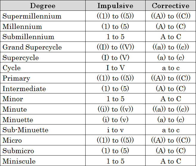
The basis of the Elliott Wave analysis is this: The market moves in a fractal pattern of waves, but the basic model is formed by an impulsive wave and a corrective wave, which, at its end, marks the beginning of another impulsive wave.

Within this idealised Elliott world, the impulsive phase is a pattern of five waves. Three of them have an impulsive nature and two have corrective.

The corrective wave pattern is composed of 3 waves, two impulsive and one corrective. Elliotticians identify them by using letters.


N.R. Elliott observed that wave patterns form larger and smaller versions of the main wave pattern. This repetition means that price behaves in a fractal manner. By keeping the wave count, traders can identify how old the current trend is and the likely place when a new one begins.


Points about Elliott Wave Analysis that helps in trading:

  1. Identifying the main trend direction.
  2. Visualising counter-trend legs.
  3. Determining the trend maturity.
  4. Defining potential targets.
  5. Specific invalidation points.


Identifying the main trend and why is it important

Impulsive waves are the easiest to trade. It’s the path of least resistance, and where reward to risk is highest. Corrective segments are hard, with a lot of volatility and noise, because it’s a place where bulls and bears fight to take control of the price. Fig 5 shows a risk to reward study on both waves, on a EUR/USD daily chart, from March to August 2015. We observe that corrective waves are noisy, with limited rewards for the risk. Impulsive waves are exuberant and optimistic, this is where we can optimise this ratio. Therefore, it’s wise to trade with the trend.

Identification of the primary trend is quite straightforward: It’s the direction pointed by one or several previous impulsive legs, in the case of Fig 5 it’s obvious we are at an uptrend.

Visualisation of Countertrend Legs

Corrective segments are places of recess from the impulsive phase. The impulse has travelled too far, according to the participants, and some of them take profits, while others sell short.

But, corrective waves are continuation patterns. Therefore, a C wave edge identifies a place of low risk and high reward to start trades aligned with the primary trend. Examples of what I mean is the end of c waves in Fig 5 that signals the beginning of a new and tradable impulsive pattern in the main trend direction.

Trend maturity determination

As we observe in Fig 4, market waves form wave patterns within wave patterns in a continuous fractal fashion. We see that wave [1] subdivides into five small waves. Therefore, we can identify the maturity of prices by looking at where they are on the wave map.

Definition of price targets

Price target assessment is done using Fibonacci ratios and one to one projections in rising channels.

Fibonacci and projections will be discussed later in more depth. On Fig 6 we see a projection example using the same EUR/USD chart from Fig 5. The line from C to 1 is copied and projected in wave 3,  starting at the end of wave 2. The length and angle are unchanged. The same projection is repeated (because wave 3 ended just as forecasted by that line) to find the end of the 5th wave. In that case, we noticed that this wave had an over-extension and this projection fell short.

The same operation can be performed on corrective waves. On Fig 6 we see an example to forecast the end levels and times of wave 4 by projecting the line drawn on wave 2.

Specific invalidation points

Knowing when the trade scenario is no longer valid is the most critical piece of information a trader needs. The wave rules give specific levels at which that scenario has failed and when the count is invalid.

Specifically, three rules help us find those invalidation levels.

  1. Wave 2 can never retrace more than 100% of wave 1.
  2. Wave 4 should never end beyond the end of wave 1.
  3. Wave 3 can never be the shortest.


A violation of these rules implies that the wave count is invalid. That will help us determine if the trade has a reward worth its risk, even before entering the trade. We should avoid less than 1:1 reward-to-risk ratios, as we have discussed in the introduction to this article.

The most profitable waves to Trade

As we have discussed before, the most profitable waves are impulsive, because they are following the direction of the primary trend.

And which waves of the total Elliott cycle are impulsive?

  • They are waves 1, 3, 5, A and C. Waves 2, 4 and B are corrective.

Particular care should be taken when trading wave 1 since the latest wave was an impulsive wave in the opposite direction, so the pattern of trend change hasn’t been established, and, usually, wave 2 corrects almost 100% of its gains. Therefore, it’s better to wait until the end of a wave 2 pullback than risking too early on a wave 1 wannabe.

We should remember that a five-wave pattern determines the direction of the main trend, while a three-wave pattern is an opportunity to join the trend.

Hence, the final count for profitable trading following the main trend are waves 3, 5, A and C.

Fig 7 shows the Elliott Wave setups. To the left, the bull market setups, while to the right the bearish market version.

As seen above, these setups, except at the end of wave 5, are entries on the main trend pullbacks, at the end of corrective waves. That makes sense because we know that impulsive waves depict much higher rewards for its risk. The second consideration is that at the end of these waves we achieve our goal to optimise the risk-reward of trades. Therefore, at least theoretically, they are as perfect an entry as they may possibly be.

Important methodology to profit from the Elliott Wave

The first rule has been already said: Trade with the trend. Just trade when a primary trend has been established.

The second rule is, let the market show you a confirmation, for example, a price breaking a strategic high or low, price breaking out of a triangle formation and so on.

The third rule has already been mentioned: We are business people. Therefore, we should seek a proper reward for our risk. We have already mentioned the importance of high reward-to-risk ratios. A ratio of 3 allows us to be profitable with just one good trade every three trades.

Let’s do an exercise. Suppose a trader has 70% success on their trades and has a reward-to-risk ratio of one. Let’s call that risk R.

After ten trades, they have won 7R and lost 3R, for a total profit of 4R.

Now suppose, we plan not to take profits so soon. For reward-to-risk ratios of 3:1, and as a consequence, we end with 40% profitable trades. Let’s do the maths:

Total profitable trades: 4 -> total profit: 3X4R= 12R

Total unprofitable trades: 6 -> total losses: 6x1R = 6R

Total Profit on ten trades = 6R

Therefore, the conclusion is clear: by planning to get 3:1 reward-to-risk ratios we are 50% more efficient, even though we decrease our hit rate by 42%. Thus, traders should take care of this primary aspect of a trade and not accept trades with less than 2:1 ratios.


Impulsive waves

The standard technique is to enter on a break of the high or low of the lower order 5th wave. This breakout defines a point of invalidation of the current trend because the last low or high has been broken.

Fig 8 shows the complete entry setups for longs and shorts. We see that the entry is executed at a breakout of wave [v] to the upside/downside, invalidating the current trend, as it failed to make new lows/highs.

Bull and bear Diagonals

According to Frost and Prechter, a diagonal is a motive pattern, but it cannot be qualified as an impulse because it holds corrective characteristics. It’s a motive because its retracements don’t fully reach the preceding sub-wave, and the third sub-wave is never the shortest. However, diagonals are the only five-wave structures in which its fourth wave moves into the price area of wave 1, and its internal waves are three-legged structures. This pattern substitutes an impulse at the corresponding location.

Ending Diagonal

An ending diagonal is a substitution of the fifth wave, usually, when the preceding move has gone too far and too fast, according to Elliott. A small percentage of diagonals appear in C-waves also. These are weak formations. According to Frost and Prechter: “Fifth wave extensions, truncated fifths, and ending diagonals all imply the same thing: dramatic reversal ahead”.

There are three ways to set up a trade on ending diagonals. The first and most conservative is to wait for the break of wave four extreme Fig 9 – (2). You gain precision at the expense of reward-to-risk ratio. You could improve that ratio by entering the trade at (1) at the breakout of the diagonal trendline connecting 2 and 4. The third way is a combination of the former two. You start taking a fractional position at (1) and, then add to the position when it breaks levels at (2).

Trading corrections

Markets movements against the primary trend are fights between those who think that the trend is over and those that see a pullback as an opportunity to jump into the trend. This struggle makes corrective patterns a dangerous and unproductive place. My advice to inexperienced traders is not to trade corrections until you get extensive knowledge about how a particular market behaves. This market phase is like to a river crowded with thousands of crocodiles. You may be lucky and cross the river, but you’re risking losing one leg or both.

A corrective phase is more complex than an impulsive phase; it unfolds slowly and depicts a noisy, random, path, taking diverse shapes such as flats, triangles zigzags or a combination. They are erratic, time-consuming, and misleading.

There are situations where the channel within which the corrective wave moves is wide enough so that the potential reward is high enough. Under those circumstances, it may be beneficial to move to a shorter timeframe to detect the right entry points.

Corrective processes show two classes. Sharp corrections and sideways channels. No more explanation needed. Sharp corrections move prices to correct a substantial part of the movement of the main trend, while sideways channels depict lateral movement that, while moving prices back the from the previous trend ending, it contains legs that carry price back to, or even beyond its initial level producing a kind of lateral channel.

There are three main categories: Zigzags, Flats and Triangles.

ZigZags

A single zig-zag in a bull market is a simple three-wave (A-B-C) pattern that pulls back some of the gains of the primary trend (fig 10, left side). In bear markets, corrections are a kind of bear traps that drive prices up in the opposite way (fig 10, right side).

On occasions, double or triple zigzags occurs. In that case, according to Frost and Prechter, zigzags are separated by an intervening “three”. These formations, still according to Frost and Prechter, are analogous to the extension of an impulse wave but are less common.

Zigzag setups for bull and bear markets are shown in Fig. 12. These setups profit from an entry at the extreme of a c-wave and assuming this is the conclusion of the correction and that a new wave in the direction of the main trend is starting.

We have three ways to trade that, as happened in ending diagonals. The more aggressive style, presenting the best reward for its risk, is taking the trade at point (1) of fig 12, which corresponds to the breakout of the [iv] sub-wave.  A more conservative approach is to wait for the breakout of the [c] wave, which also corresponds to the extreme of wave B (Fig. 12, point (2)). Finally, we could take a medium-risk approach by opening with a fraction of the total risk at (1) and take the rest at (2).

Flats

A flat is a correction that differs from a zigzag in that its sequence is a 3-3-5 wave. The reason is that the first wave A lacks the strength to create five sub-waves. Then B-wave finishes near the starting of A and then C, having five sub-waves that generally, ends slightly below A, almost drawing a double bottom or top.

The final wave of a flat wave is a 5-wave pattern. Therefore, we can apply the setup used for the 5th wave (Fig. 8). That means trading the breakout of the [iv]sub-wave. Fig 14 shows the configuration for bull and bear markets.


Triangles

A triangle is a price pattern reflecting doubts and a balance of opinions between market participants. This pattern subdivides into 3-3-3-3-3 sub-waves, labelled A, B, C, D, and E. A triangle is outlined when connecting A and C, and B and D. It’s usual for Wave E to undershoot or overshoot the A-C line.

There are three triangle varieties: Contracting, barrier and expanding.

The safest entry waits for wave [c] wave to be broken. More aggressive entries are not recommended because triangles are very deceptive, and sometimes some formation that seems a bullish continuation pattern actually could become a bearish triangle.


This completes this basic guide to Elliott Wave trading. In upcoming articles, we will examine real chart examples of the setups sketched out in this document.


References:

Visual guide to Elliott Wave Trading, Wayne Gorman

Elliott Wave Principle: Key to Market Behavior, Robert R. Prechter Jr.; A. J. Frost.


© Forex. Academy