This is a small presentation about how, at Forex Academy, you could discover the secrets behind risk control; and how position size could affect your profits and your probability of ruin.
Forex Academy’s Educational Library consists of the finest collection of written and video pieces of learning material. It focuses on every relevant aspect of trading.
This is a small presentation about how, at Forex.Academy, you could discover the secrets behind risk control; and how position size could affect your profits and your probability of ruin.

This is a small presentation about how, at Forex.Academy, you could discover the secrets behind risk control; and how position size could affect your profits and your probability of ruin.
This is a small presentation about how, at Forex Academy, you could discover the secrets behind risk control; and how position size could affect your profits and your probability of ruin.
The AUDUSD pair in daily chart is moving bearish as an A-B-C pattern, from the highest level reached on January 25 (0.81358 level). The segment BC developed a bullish divergence, which alerts us to the exhaustion of the bearish movement, this divergence is not a reversal signal. On the last sequence of the wave C, the price tested two times the 0.73179 level (FE 141.4 level).
In the 4-hour chart, the wave between B and C has fallen in five waves from 0.79163 to 0.73105 on July 02. From this level, the Aussie started an internal bullish move which reached the 0.74838 level, surpassing the previous high 0.74438 in time and shape. Currently, the price is moving in a range which could be the start of a new bullish cycle.
For the coming sessions, we foresee new upsides which could be activated as long as the price bounce from the area between 0.73562 and 0.73265, with a potential profit target area between 0.75382 and 0.75956. The invalidation level of this scenario is 0.73105.
Forex Daily News: In this post, we analyse the Canadian Dollar group against their main currencies. As a summary, the second half of the year and 2019, we foresee a corrective movement in the Canadian currency, which could come supported for a correction in oil prices to, then, give way to a new rally. After this correction, our central vision for the Canadian Dollar is a new appreciation scenario.
Additionally, we observe that it is likely that GBP and EUR would show the best performance against the CAD; on the opposite side, the Japanese currency and the Swiss Franc could have the worst performance against the Canadian Dollar.
The USDCAD is developing a complex corrective structure of a second bullish impulsive wave. The corrective structure has a bearish bias, which could find support in the area between 1.29607 to 1.28371. The key level to watch out is 1.2884, this level should convert on a critical pivot level (HHL).
EURCAD cross in the short-term has a bearish bias, probably could see new lows in 1.50 zone. In the mid-term, the cross moves sideways as a complex corrective. In the long-term, we foresee that the EURCAD could find fresh lows in the area between 1.47822 to 1.45662, from where the cross could start a new rally as a fifth bullish wave. Invalidation level is at 1.4442.
Probably the GBPCAD cross shows the clearest movement of the CAD Group. The price is moving in a bearish A-B-C sequence, which could find support at 1.6410 level, from where the price could create a new connector and then initiate a rally. The new bullish sequence has a target the area between 1.8533 and 1.9266. Invalidation level is at 1.5837.
The CADJPY cross has been commented in a previous analysis, and we maintain the main idea which consists in to seek only long positions with a long-term profit target in the area between 94.69 and 95.30. Is probably that the cross makes a retrace to the area between 85.45 to 83.73 from where we could find new opportunities to incorporate us into the trend. Invalidation level is located at 82.17.
In the CADCHF cross, the lemma is “Buy the Dips” or “Watch the Breakout.” CADCHF is running sideways in an upper degree consolidation structure. The key level to control is 0.7636, after the breakout of this level, we expect more upsides to the zone between 0.7992 and 0.8245. In case that the price makes a false breakdown to the area between 0.7394 and 0.7289, it could be an attractive opportunity to look for the long side. Invalidation level is at 0.7124.
In the long-term, NZDCAD is running sideways and making lower highs. The long-term pivot level is at 0.8640. For this cross, we expect only short positions; if the price makes a bullish move, the potential movement is limited to the area between 0.9253 to 0.9461. The long-term target area is between 0.8401 to 0.8098.
Probably the AUDCAD cross is the less attractive to trade. As we can see in the weekly chart, it is running sideways since the second half of 2013. The price is moving inside a bearish cycle, which could find support in the “long-term pivot level” at 0.8919, from where AUDCAD could start to bounce. The invalidation level for the bearish cycle is at 1.0397.
Forex Daily News: Finally, as a technical note, considering that the AUDCAD is mostly bearish, by correlation, the CAD should perform better than the AUD for the period foreseen.
Introduction
Traders want to win. Nothing else matters to them; and they think and believe the most important question is timing the entry. Exits don’t matter at all, because if
Introduction
Traders want to win. Nothing else matters to them; and they think and believe the most important question is timing the entry. Exits don’t matter at all, because if
Traders want to win. Nothing else matters to them; and they think and believe the most important question is timing the entry. Exits don’t matter at all, because if they time the entry, they could easily get out long before a retracement erases their profit. O so they believe.

That’s the reason there are thousands of books about Technical Analysis, Indicators, Elliott Wave Forecasting, and so on, and just a handful of books on psychology, statistical methods, and trading methodology.
The problem lies within us, not in the market. The truth is not out there. It is in here.
There are a lot of psychological problems that infest most of the traders. One of the most dangerous is the need to be right. They hate to lose, so they let their losses run hoping to cover at a market turn and cut their gains short, afraid to lose that small gain. This behavior, together with improper position sizing is the cause of failure in most of the traders.
The second one is the firm belief in the law of small numbers. This means the majority of unsuccessful traders infer long-term statistical properties based on very short-term data. When his trading system enters in a losing streak, they decide the system doesn’t work, so they look for another system which, again, is rejected when it enters in another losing sequence and so on.
There are two problems with this approach. The first one is that the trading account is constantly consumed because the trader is discarding the system when sits at its worst performance, adding negative bias to his performance every time he or she switches that way. The second one is that the wannabe trader cannot learn from the past nor he can improve it.
This article is a rough approach to the problem of establishing a trading methodology.
1.- Diversification
The first measure a trader should take is:
What’s the advantage of a diversified portfolio:
The advantage of having a diversified portfolio of assets is that it smooths the equity curve and, and we get a substantial reduction in the total Drawdown. I’ve experienced myself the psychological advantage of having a large portfolio, especially if the volatility is high. Losing 10% on an asset is very hard, but if you have four winners at the same time, then that 10% is just a 2% loss in the overall account, that is compensated with, maybe, 4-6% profits on other securities. That, I can assure you, gave me the strength to follow my system!.
The advantage of three or more trading systems in tandem is twofold. It helps, also improving overall drawdown and smooth the equity curve, because we distribute the risk between the systems. It also helps to raise profits, since every system contributes to profits in good times, filling the hole the underperforming one is doing.
That doesn’t work all the time. There are days when all your assets tank, but overall a diversified portfolio together with a diversified catalog of strategies is a peacemaker for your soul.
2.- Trading Record
As we said, deciding that a Trading System has an edge isn’t a matter of evaluating the last five or ten trades. Even, evaluating the last 30 trades is not conclusive at all. And changing erratically from system to system is worse than random pick, for the reasons already discussed.
No system is perfect. At the same time, the market is dynamic. This week we may have a bull and low volatility market and next one, or next month, we are stuck in a high-volatility choppy market that threatens to deplet our account.
We, as traders need to adapt the system as much as is healthy. But we need to know what to adjust and by how much.
To gather information to make a proper analysis, we need to collect data. As much as possible. Thus, which kind of data do we need?
To answer this, we need to, first look at which kind of information do we really need. As traders, we would like to data about timing our entries, our exits, and our stop-loss levels. As for the entries we’d like to know if we are entering too early or too late. We’d like to know that also for the profit-taking. Finally, we’d like to optimize the distance between entry and stop loss.
To gather data to answer the timing questions and the stop loss optimum distance the data that we need to collect is:
All the above concepts are well known to most investors, except, maybe, the two bottom ones. So, let me focus this article a bit on them, since they are quite significant and useful, but not too well known.
MAE is the maximum adverse price movement against the direction of the trend before resuming a positive movement, excluding stops. I mean, We take stops out of this equation. We register the level at which a market turn to the side of our trade.

MFE is the maximum favourable price movement we get on a trade excluding targets. We register the maximum movement a trade delivers in our favour. We observe, also, that the red, losing trades don’t travel too much to the upside.

Having registered all these information, we can get the statistical evidence about how accurate our entry timing is, by analysing the average distance our profitable trades has to move in the red before moving to profitability.
If we pull the trigger too early, we will observe an increase in the magnitude of that mean distance together with a drop in the percent of gainers. If we enter too late, we may experience a very tiny average MAE but we are hurting our average MFE. Therefore, a tiny average MAE together with a lousy average MFE shows we need to reconsider earlier entries.
We can, then, set the invalidation level that defines our stop loss at a statistically significant level instead of at a level that is visible for any smart market participant. We should remember that the market is an adaptive creature. Our actions change it. It’s a typical case of the scientist influencing the results of the experiment by the mere fact of taking measurements.
Let’s have a look at a MAE graph of the same system after setting a proper stop loss:

Now All losing trades are mostly cut at 1.2% loss about the level we set as the optimum in our previous graph (Fig 2). When this happens, we suffer a slight drop in the percent of gainers, but it should be tiny because most of the trades beyond MAE are losers. In this case, we went from 37.9% winners down to 37.08% but the Reward risk ratio of the system went from results 1.7 to 1.83, and the average trade went from $12.01 to $16.5.
In the same way, we could do an optimization analysis of our targets:

We observed that most of the trades were within a 2% excursion before dropping, so we set that target level. The result overall result was rather tiny. The Reward-to-risk ratio went to 1.84, and the average trade to 16.7
These are a few observations that help us fine-tune our system using the statistical properties of our trades, together with a visual inspection of the latest entries and exits in comparison with the actual price action.
Other statistical data can be extracted from the tracking record to assess the quality of the system and evaluate possible actions to correct its behaviour and assess essential trading parameters. Such as Maximum Drawdown of the system, which is very important to optimize our position size, or the trade statistics over time, which shows of the profitability of the system shrinks, stays stable or grows with time.

This kind of graph can be easily made on a spreadsheet. This case shows 12 years of trading history as I took it from a MACD trading system study as an example.
Of course, we could use the track record to compute derived and valuable information, to estimate the behaviour of the system under several position sizes, and calculate its weekly or monthly results based in the estimation, along with the different drawdown profiles shaped. Then, the trader could decide, based upon his personal tolerance for drawdown, which combination of Returns/drawdown fit his or her style and psychological tastes.
The point is, to get the information we must collect data. And we need information, a lot of it, to avoid falling into the “law of small numbers” fallacy, and also to optimize the system and our risk management.
Note: All images were produced using Multicharts 11 Trading Platform’s backtesting capabilities.
The Nature of Risk and Opportunity
Trading literature is filled with vast amounts of information about market knowledge: fundamentals, Central Banks, events, economic developments and technical analysis. This information is
The Nature of Risk and Opportunity
Trading literature is filled with vast amounts of information about market knowledge: fundamentals, Central Banks, events, economic developments and technical analysis. This information is
Trading literature is filled with vast amounts of information about market knowledge: fundamentals, Central Banks, events, economic developments and technical analysis. This information is believed necessary to provide the trader with the right information to improve their trading decisions.
On the other hand, the trader believes that success is linked to that knowledge and that a trade is good because the right piece of knowledge has been used, and a bad trade was wrong because the trader made a mistake or didn’t accurately analyse the trading set-up.
The focus in this kind of information leads most traders to think that entries are the most significant aspect of the trading profession, and they use most of their time to get “correct” entries. The other consequence is that novice traders prefer systems with high percent winners over other systems, without more in-depth analysis about other aspects.
The reality is that the market is characterized by its randomness; and that trading, as opposed to gambling, is not a closed game. Trading is open in its entry, length, and exit, which gives room for uncountable ways to define its rules. Therefore, the trader’s final equity is a combination of the probability of a positive outcome – frequency of success- and the outcome’s pay-off, or magnitude.
This latest variable, the reward-to-risk ratio of a system, technically called “the pay-off” but commonly called risk-reward ratio, is only marginally discussed in many trading books, but it deserves a closer in-depth study because it’s critical for the ultimate profitability of any trading system.
To help you see what I mean, Figure 1 shows a game with 10% percent winners that is highly profitable, because it holds a 20:1 risk-reward ratio.

A losing game is also possible to achieve with 90% winners:

So, as we see, just the percentage winners tell us nothing about a trading strategy. We need to specify both parameters to assess the ultimate behaviour of a system.
Let’s call Rr the mean risk-reward of a system. If we call W the average winning trade and L the average losing trade then Rr is computed as follows:
Rr = W/L
If we call minimum P the percent winners needed to achieve profitability, then the equation that defines if a system is profitable in relation to a determined reward-risk ratio Rr is:
P > 1 / (1 +Rr) (1)
Starting from equation (1) we can also get the equation that defines the reward-risk needed to achieve profitability if we define percent winners P:
Rr > (1-P) / P (2)
If we use one of these formulas on a spreadsheet we will get a table like this one:

When we look at this table, we can see that, if the reward is 0.5, a trader would need two out of three winning trades just to break-even, while they would require only one winner every three trades in the case of a 2:1 payoff, and just one winner every four trades if the mean reward is three times its risk.
Let’s call nxR the opportunity of a trade, where R is the risk and n is the multiplier of R that defines the opportunity. Then we can observe that:
A high Rr ratio is a kind of protection against a potential decline in the percentage of winning trades. Therefore, we should make sure our strategies acquire this kind of protection. Finally, we must avoid Rr’s under 1.0, since it requires higher than 50% winners, and that’s not easy to attain when we combine the usual entries with stop-loss protection.
One key idea by Dr. Van K. Tharp is the concept of the low-risk idea. As in business, in trading, a low-risk idea is a good opportunity with moderate cost and high reward, with a reasonable probability to succeed. By using this concept, we get rid of one of the main troubles of a trader: the belief that we need to predict the market to be successful.
As we stated in point 3 of lessons learned: we don’t need to predict. You’ll be perfectly well served with 20% winners if your risk reward is high enough. We just need to use our time to find low-risk opportunities with the proper risk-reward.
We can find a low-risk opportunity, just by price location as in figure 3. Here we employ of a triple bottom, inferred by three dojis, as a fair chance of a possible price turn, and we define our entry above the high of the latest doji, to let the market confirm our trade. Rr is 3.71 from entry to target, so we need just one out of four similar opportunities for our strategy to be profitable.

Finally, we should use Rr as a way to filter out the trades of a system that don’t meet our criteria of what a low-risk trade is.
If, for instance, you’re using a moving average crossover as your trading strategy, by just filtering out the low profitable trades you will stop trading when price enters choppy channels.
As we observe in Fig 3, the risk is defined by the distance between the entry price and the stop loss level, and the reward is the distance between the projected target level defined by the distance from the Take profit level to the entry price:
Risk = Entry price– Stop loss
Reward = Take profit – Entry price.
Rr = Reward / Risk
In this case,
Entry price = 1.19355
Stop loss = 1.19259
Take profit = 1.19712
Therefore,
Risk = 1.19355 -1.19259 = 0.00096
Reward = 1.19712 – 1.19355 = 0.00357
Rr = 0.00357 / 0.00096
Rr = 3.7187
©Forex.Academy
In this editorial we are going to discuss decentralized exchanges, why they exist or why are they going to exist, what are the advantages, what aren’t people still using them, and we will have an overview of the current projects that are striving to solve these problems.
Let’s start off with explaining how normal (centralized exchanges) work and what’s their purpose. This will serve as an introduction to the problem which decentralized exchanges tend to solve.
Centralized exchanges act as a third party matchmaker between a buyer and a seller of an asset. They are useful because they provide liquidity. What is also important is that this process of trading is speeded up by the convenience of having an account in which you have you deposited funds, which are held by the exchange.
>Liquidity describes the degree to which an asset or security can be quickly bought or sold in the market without affecting the asset’s price.
Market liquidity refers to the extent to which a market, such as a country’s stock market or a city’s real estate market, allows assets to be bought and sold at stable prices. Cash is considered the most liquid asset, while real estate, fine art, and collectibles are all relatively illiquid.
Accounting liquidity measures the ease with which an individual or company can meet their financial obligations with the liquid assets available to them. There are several ratios that express accounting liquidity highlighted below.
Source: investopedia.com
The most popular examples of centralized cryptocurrency exchanges are: Coinbase, Kraken, Cex, Bitfinex, Poloniex…
In the cryptocurrency market exchanges are often divided into two types: fiat-crypto gateway (BTC/USD, ETH/USD, LTC/USD…) and altcoins (BTC/ZRX, BTC/DNT, ETH/ADA…)
This is important to point out because later we will discuss some common problems associated with decentralized exchanges (DEX) that are caused by these points.
Unlike centralized exchanges, DEXs aren’t owned by anyone. Instead, they are constructed on the same distributed ledger technology as Bitcoin and utilize smart contracts for order execution. This is important to point out, as this means that they do not hold funds for their beneficiaries or any other relevant information regarding the identity or location.
Some common examples are: Etherdelta, IDEX, Radar Relay.
Centralized exchanges are charging high fees, which is something cryptocurrencies strive to eliminate. They can be hacked which happened numerous time in the past. They have the ownership of your funds, which is something that’s not aligned with the advantages of cryptocurrencies in general (cryptos take pride in the part that people have control of their own money). Crypto-unfriendly governments can cut or ban their operations. For all the above reasons they are viewed as the weakest link in the cryptocurrency market ecosystem.
That’s why decentralized exchanges are offered as a solution to the listed problems. They cannot be hacked, they cannot be tampered with, they are censorship resistant and do not hold your funds.
While DEXs are more beneficial when it comes to security (from hackers and government interference), anonymity and cost, there are still great challenges that they need to overcome in order to compete with their centralized competition. They are still difficult to use for the common person, as you would have to be crypto/tech savvy; they are somewhat limited in functionality and/or limited on the type of a cryptocurrency (for example only ERC20 tokens), and most importantly they don’t guarantee liquidity.
Having liquidity and a large trading volume is most important because we as traders are all about fast execution. And if you have to wait for hours for your order to get filled, by the time you might get fill you aren’t potentially looking at a good buy or sell opportunity.
Because of this, DEXs haven’t been much used, compared to their centralized counterpart. But there are projects out there that are going to solve that problem as well. In the following paragraphs, we will review most promising DEX projects.
0x is a protocol. That means it serves as a layer on top of the Ethereum blockchain for actually building decentralized exchange applications. They describe in their whitepaper that 0x is “a protocol that facilitates low friction peer-to-peer exchange of ERC20 tokens on the Ethereum blockchain. The protocol is intended to serve as an open standard and common building block, driving interoperability among decentralized applications (dApps) that incorporate exchange functionality. Trades are executed by a system of Ethereum smart contracts that are publicly accessible, free to use and that any dApp can hook into. DApps built on top of the protocol can access public liquidity pools or create their own liquidity pool and charge transaction fees on the resulting volume.”
OmiseGO is a project that incorporates many things, but having in mind the focus of this editorial we are going to point out their dex platform.
“OmiseGO is building a decentralized exchange, liquidity provider mechanism, clearinghouse messaging network, and asset-backed blockchain gateway. OmiseGO is not owned by any single one party. Instead, it is an open distributed network of validators which enforce behavior of all participants. It uses the mechanism of a protocol token to create a proof-of-stake blockchain to enable enforcement of market activity amongst participants. This high-performant distributed network enforces exchange across asset classes, from fiat-backed issuers to fully decentralized blockchain tokens (ERC-20 style and native cryptocurrencies). Unlike nearly all other decentralized exchange platforms, this allows for decentralized exchange of other blockchains and between multiple blockchains directly without a trusted gateway token.”
Source: OmiseGO whitepaper
Airswap is similar to 0x in a sense that it will allow users to exchange only ERC20 tokens, and in a sense that it’s a consensus project. The difference is that the transaction on Airswap happens off the chain.
“We present a peer-to-peer methodology for trading ERC20 tokens on the Ethereum blockchain. First, we outline the limitations of blockchain order books and offer a strong alternative in peer-to-peer token trading: off-chain negotiation and on-chain settlement. We then describe a protocol through which parties are able to signal to others their intent to trade tokens. Once connected, counterparties freely communicate prices and transmit orders among themselves. During this process, parties may request prices from an independent third party oracle to verify accuracy. Finally, we present an Ethereum smart contract to fill orders on the Ethereum blockchain.”
Source: Airswap whitepaper
Kyber network is my favorite project as they tend to emulate the exact same functionalities and user experience as centralized exchanges.
We design and build KyberNetwork, an on-chain protocol which allows instant exchange and conversion of digital assets (e.g. crypto tokens) and cryptocurrencies (e.g. Ether,
Bitcoin, ZCash) with high liquidity. KyberNetwork will be the first system that implements several ideal operating properties of an exchange including trustless, decentralized execution, instant trade and high liquidity.
The only thing that’s different is that they don’t have the order book in order to finally solve the liquidity issue.
Instead of maintaining a global order book, we maintain a reserve warehouse which holds an appropriate amount of crypto tokens for purposes of maintaining exchange liquidity. The reserve is directly controlled by the Kyber contract, and the contract has a conversion rate for each exchange pair of tokens by fetching from all the reserves. The rates are frequently updated by the reserve managers, and Kyber contract will select the best rate for the users. When a request to convert from token A to token B arrives, the
Kyber contract checks if the correct amount of token A has been credited to the contract, then sends the corresponding amount of token B to the sender’s specified address. The
amount of token A, after the fees, is credited to the reserve that provides the token B.
Source: Kyber Network whitepaper
Having experienced these problems of centralized exchanges early on, cryptocurrency ecosystem has already come up with the solution – decentralized exchange applications. They are still far from perfect but as you can see from these promising examples, some major obstacles are already being solved as well. First generation failed but offered a great insight on how and where to look for progress. That’s the beauty of the free market – problems are being solved and those who can’t compete are left behind.
The greatest threat of centralized exchanges aren’t the reasons I’ve listed. The greatest power centralized exchanges have is maker manipulation. They collect so many cryptos through fee’s that they can manipulate the price in many ways. They also have awareness of the order book flow that they can use to their advantage.
Something like that happened on October 8. last year on Bittrex exchange. Even though they denied the accusations of market manipulation, the research done by The CryptoSyndicate Research Lab paint a different story.
For more check out the original post:
https://thecryptosyndicate.com/opinion-bittrex-anomaly/
In the spirit of decentralization which cryptocurrencies carry and promise, in order to achieve taking power back from centralized entities, decentralized exchanges are emerging widely. It is up to us to choose what’s best for us, so I have not doubt in my mind that DEXs will become a new standard in the near future, but only after they offer easy user experience and liquidity.
Having said that, and having in mind the projects that are already out there, “near future” may be sooner than we think.
©Forex.Academy
Cryptocurrency market is still in its infancy stage. That means that the industry around it is too. People all around the world are jumping at the opportunity to take the piece of the pie, and whoever gets it first is his. This results in a great influx of financial layman’s offering advice, bringing news and teaching you how to trade, especially on youtube where people first come for information because it’s easier to accept it in a video format.
A sentence I commonly hear among those who offer this information is: This is not financial advice, do your own research. They say this in order to legally protect themselves, yet they do offer financial advice. That’s why doing your own due diligence in the cryptocurrency market is crucial. And to assist you in that I’ve created a template for you to evaluate your source of information.
I’ve divided them into three categories: news, ico’s and analysis.
Regarding news:
1.1 Is it a direct source (e.g., projects website or other social media outlets such as medium, (sub)Reddit, Twitter) (good)
1.2 Is it indirect source (news website) (neutral)
2.1 Entertainment (neutral)
2.2 To inform (good)
2.3 Advertisement and/or interest (bad)
Your goal should be to be the closest to the source as possible. If you are interested in latest developments of your favourite crypto project, join their telegram group, or slack channel. Every established project has one. If not go to Reddit and find their subreddit, where admins are the official community managers for the project. Many of them also have a blog on Medium where they update their readers on a regular basis.
Regarding ICO recommendation:
1.1 Does it come from someone within the space (good)
1.2 Does it come from someone outside the space (neutral)
2.2.1 To promote because of his interest (bad)
2.2.1 Is it just a fresh topic (neutral)
2.2.3 Because he believes it’s a good idea (good)
Cross-reference that will other people recommending the same thing, and/or ask people for their opinion.
As an example, you don’t want to take your ICO recommendations from the CNBC’s show Crypto Trader. Why? Because those are sponsored, and the show is for entertainment purposes.
Analysis:
1.1 Success track record:
1.1.1 no track record (bad)
1.1.2 vague track record (neutral)
1.1.3 clear track record (good)
1.2 Prior (before crypto) engagement in financial markets
1.2.1 yes (good)
1.2.2 no (bad)
2.1 Only crypto market (neutral)
2.2. Broad understanding of financial markets (good)
In the crypto world, everybody’s a trader or knows a thing or two about technical analysis. And that’s a good thing, but chose carefully who you are listening to when it comes to putting your money on the line. Ideally, you shouldn’t be listening to anybody. You should learn how to do your own analysis or higher a certified financial analyst to consult you on your investments.
That’s it. Now next time you are searching for information you have a way to validate them. I encourage you to expand on this template and create your own. Incorporate things that you find important when it comes to evaluating your source. And remember: always do your own research.
Novice traders enter the Forex markets with the illusion of becoming independent and wealthy. And they may be right. So why 95% of forex traders fail?
After no trading
Novice traders enter the Forex markets with the illusion of becoming independent and wealthy. And they may be right. So why 95% of forex traders fail?
After no trading
Novice traders enter the Forex markets with the illusion of becoming independent and wealthy. And they may be right. So why 95% of forex traders fail?
After no trading plan and psychological weaknesses and biases comes Too high position sizing as the main cause for failure.
I guess that the become rich quick mentality, an evident psychological weakness, drives them to trade big at the wrong time. Then Fear and greed make the rest.
Therefore, my first recommendation for a new trader is to doubt about his strength to support the psychological pressure to break his system. That is much better accomplished if he or she risks small amounts. The initial two years of trading should be dedicated to learn and practice the needed discipline to respect the trading rules.
To help you take out your anxiety for a quick buck profit, Let’s analyse the power of compounding.
Let’s first see, graphically an account of 10,000 € grow at a monthly rate of 0,083%, a nominal annual rate of 1% for 50 years (600 months):

Well, we observe that this state of affairs is only good for the bankers. It takes 50 years to grow 10K into 16,500K. That’s the reason we are willing to risk trading.
Let suppose we get a risk-free 10% annual return instead, again, with monthly payments of 10%/12:

That is becoming interesting. One, we need to wait patiently for 50 years to become millionaires, and, two, we don’t know how much of that will be erased by inflation.
Let’s suppose we are investing ala Warren Buffett with an annual mean return of 26%, that, also steadily grows on a monthly basis. In this case, the graph is presented in semi-log scale for obvious reasons. The x-scale is in months while the y-scale says how many zeros has the account balance. For instance, 106 means the account has 1 followed by six zeros:

Now, that is another history! We see that in 50 years we will be as filthily rich as Warren Buffett et al. ! We observe, also, that we add one zero to our account roughly once every 100 months. Not Bad. We multiply by ten our stake every two years! And that is achieved with a mean monthly rate of return on our capital of 2.17%, which means we just need to make sure we get a daily return of 0.11%.
The problem is within us:

This one is the same equity curve than the previous one but in a linear scale. We observe that it shows an exponential line, and there resides our psychological problem: The net equity grows relatively slow at the beginning. We need four years to reach six zeros, but in another four years, we will be close to eight. That shows that the power of compounding is a long-distance race, not a sprint.
Things are not that perfect in trading. We don’t see nice curves up to richness. We should expect not only run-ups but, also drawdowns. Let’s observe the equity curve of a typical system using a nominal risk of 0.5% which takes, for simplicity, one trade per day, or 20 per month. And let’s put a magnifying glass on the first year of its history.

   Starting Capital:  10,000
Mean ending Capital:  11,817
     Capital % gain:  18.17%
       Max drawdown:  2.64%

This is a real system, achievable, with the basic statistics as follows:
STRATEGY STATISTICS:
              Nr. of Trades: 143.00
                    gainers: 58.74%
              Profit Factor: 1.74
                   mean nxR: 1.22
 Sample Stats Parameters:
           mean(Expectancy): 0.3070
               Standard dev: 1.9994
            VAN K THARP SQN: 1.5353
The monthly mean profit, using a 0.5% risk is 1.5%, which gives an annual growth of 18%. A bit less than what Warren Buffet has been performing. The nice feature is that using a 0.5% risk the max drawdown is 2.64%. Now, let’s see how fare this system, using exactly the same trade percent results when risk rises because we increase the position size:

   Starting Capital:  10,000
Mean ending Capital:  18,910
     Capital % gain:  89.10%
       Max drawdown:  10.38%
5% risk:
     Starting Capital:  10,000
  Mean ending Capital:  42,615
       Capital % gain:  326.15%
         Max drawdown:  25.39%
10% Risk:
     Starting Capital:  10,000
  Mean ending Capital:  118,032
       Capital % gain:  1,080.32%
         Max drawdown:  47.67%
20% Risk:
     Starting Capital:  10,000
  Mean ending Capital:  308,888
       Capital % gain:  2,988.88%
         Max drawdown:  79.99%
35% Risk:
   Starting Capital:  10,000
Mean ending Capital:  124,613
     Capital % gain:  1,146.13%
       Max drawdown:  96.83%
45% Risk:

   Starting Capital:  10,000
Mean ending Capital:  14,725
     Capital % gain:  47.25%
       Max drawdown:  99.53%
From the above examples we take that:
A simple approach to compute the preferred risk per position is to be prepared for a 10-15 consecutive losing streak.
Let’s suppose we want our drawdown to be limited to 20%. If our system statistics show that our percent winners are less than 50%, then we should be protected to at least 15 losers in a row. If our percent winners stats are above 50% and our mean reward-to-risk ratio is above 1, then we may settle for ten losers in a row.
The method to limit the risk is easy. We divide the drawdown amount by the losing streak number.
If we wanted to be protected of a 20 losing streak and our maximum decided drawdown is 20% then, 20%/20 tells us that we cannot risk more than 1% on each trade. In the case of a 15 losing streak, our max risk goes to 1.33%, and it goes to 2 in the case of a 10 figure.
Therefore, If you trade using 0.5% risk on your account, you make sure that your maximum drawdown halves, therefore it’s highly improbable that your drawdown moves above 10% of your current balance.
Below is a possible 30-year history of the sample system using 0.5% risk. Sometimes, the turtle wins to the rabbit, because a too fast rabbit may get hit by a bullet.

The information received by the Federal Open Market Committee (FOMC), since its meeting in January, has shown signs of further strengthening of the labour market and economic activity has been growing at moderate but solid rates. Job gains have grown strong in recent months, and the unemployment rate has remained at low levels. Recent data shows that the growth rate of household spending and business fixed investment has grown in 2018 at moderate rates after a large growth at the end of 2017.
On a twelve-month basis, overall inflation and inflation for items other than food and energy has remained below 2%. The economic outlook has improved in recent months due to the good results evidenced throughout 2017, and since the tax reform approved at the end of the same year.
The committee expected that with gradual adjustments in the monetary policy stance, the economy would continue to behave positively in the medium term and labour market conditions would remain robust. Regarding inflation and its annual base, the committee expected that in the short term this indicator would be close to 2% and that the bank’s goal would be met.
Due to the behaviour of the labour market, the main sectors of the economy and inflation, the committee decided to raise the target range of federal funds from 1.5% to 1.75%. The committee was explicit in that the monetary policy stance would remain accommodative as long as it was necessary for inflation to return to 2%.
This decision was in line with market expectations, so there was no strong reaction from the market. In the projections of the path of the interest rate, there is still no unanimity on what the next steps of the Federal Reserve will be as some expect a stronger policy, so they expect four increases during 2018. For other analysts, the path will continue the road stipulated so they expect only three increases during the current year.
The following graph shows the main projections of the committee. This graph shows economic growth above the natural long-term rate and the rates expected since the December meeting has improved. The unemployment rate also shows a very positive behaviour and is below the long-term rate. Regarding the different inflation measures, inflation is expected below the bank’s target for 2018, but very close to the target level, and for the next two years, an optimal inflation rate is expected according to the bank’s mandate.

Graph 82.Economic projections of Federal Reserve Board members and Federal Reserve Bank presidents, March 2018. Retrieved 23rd March 2018 from https://www.federalreserve.gov/monetarypolicy/files/monetary20180321a1.pdf
In the press conference, the president of the Federal Reserve Jerome Powell expressed that the decision to raise the target range of the interest rate marks another step in the normalisation of monetary policy, a process that has been underway for several years. But in his statements, some caution was evident and showing that the path of the interest rate considered only two more hikes in 2018.
Job gains averaged 240,000 per month in the last three months, which is a very positive rate and makes it possible for new workers to be absorbed. The unemployment rate remained at low rates in February, standing at 4.1%, while the rate of labour market participation increased.
According to Powell, that is a positive signal given that the economically active population is getting older, so this leads to the participation rate to the downside, but with the new entries this negative effect is offset by the entry of new workers.
Also, the president of the Federal Reserve has concluded that there are certain specific factors that have contributed to the greater economic growth observed in recent months and these are:
Regarding inflation, Powell was clear that inflation was still below 2% regardless of what measure was used. According to the president of the Federal Reserve, this was due to unusual price reductions that occurred in late 2016 and early 2017. But for Powell, as the months passed in 2018, these unusual events would disappear, and inflation would be very close to 2 %.
In his statements, the president of the Federal Reserve specified that, if the rates rose too slowly, this would increase the risk that monetary policy would have to adjust abruptly in the future if a shock should occur in the economy. At the same time, the committee wanted to prevent inflation from remaining below the target which could reduce the chances of acting quickly in the face of a recession in the US economy.
Finally, Powell pointed out that the reduction in the balance sheet that began in October was progressing smoothly. Only specific conditions of the economy could curb the normalisation of the balance sheet of the Federal Reserve. President Powell was emphatic that they would use the balance sheet in addition to the interest rate to intervene in the economy if a deep economic recession were to occur.
In conclusion, the federal committee decided to raise the federal funds rate as expected by the market due to the good performance of the economy which continued to grow at high rates and above the long-term level. Although inflation was not at the desired level, according to the committee, this was due to transitory effects that would fade over the months, and thus inflation would be in the target range.
As already mentioned, the economy showed good signs due to the labour market, so the bank decided to raise rates, but the committee remained cautious about the future of the economy because it was not ruled out that a recession would occur. According to the statements made at the press conference, some indecision was evident on the part of the committee as they evaluated the two possible scenarios against the interest rate.
If they raised it too quickly they could slow down the economy and thereby affect the labour market, which would lead to a drop in inflation, which would lead to a complex economic scenario as future increases would not be possible, and this would restrict the use of the monetary policy. On the contrary, If the committee raised it too slowly, a scenario could be generated where any economic shock, whether internal or external, could also affect the economic growth of the United States and limit future increases in the interest rate.
The market is still undecided if the FED will make two or three more rate hikes during the current year. Some analysts question why the Federal Reserve continues to raise rates if the inflation rate still shows no stability. For them, the central bank should be more cautious in its monetary policy because they could be in the second scenario where the economy still needs an accommodative policy so that the medium term could be limited future increases in the rate as well as the normalisation of the balance sheet.
Category: Fundamental Analysis, Intermediate, Currencies, economic cycles, Monetary Policy, Economy, Macroeconomics, Central Banks.
Key Words: Central Banks, Monetary Policy, Bank of Japan.
Tags: Macroeconomy, BoJ, Monetary policy, 2017.
At the January 2016 meeting, the Central Bank of Japan introduced negative interest rates, setting the reference rate at 0.1%. This negative rate meant that the central bank would charge commercial banks for some reserves deposited in Japan’s central financial institution. The measure was designed to encourage commercial banks to use their reserves to increase the supply of loans to consumers and investors in Japan, to reactivate the economy and overcome the deflation that the country was experiencing at that time.
This negative rate would not apply directly to the accounts that customers had with commercial banks so as not to affect the purchasing power of individuals or companies. It was not a measure taken impulsively since the Bank of Japan had been analysing what measures could boost the behaviour of inflation for several years.
The decision was made by the board of the bank in a split decision of 5 votes in favour of the measure, against four votes who did not agree to establish negative rates. In addition, the report issued summarising the meeting, stipulated that if it was necessary to delve into the negative rates territory, this measure would be only be implemented until the bank achieved its 2% goal.
This measure of establishing negative rates has not been common for the central banks of the world’s leading economies since there is no consensus on the possible effects of negative rates. A problem that had lasted for quite some time in Japan was the decline in the prices of goods and services so that consumers restricted their spending due to their expectations of prices in the future.
At the press conference, the governor of the Bank of Japan, Haruhiko Kuroda indicated that deflation coupled with a global economic slowdown led to an unprecedented policy for Japan. For many analysts, the decision to adopt negative rates was surprising, and it was not known how much this could influence the short and medium-term inflation rate.
The consensus for many analysts was that the Japanese economy did not grow at higher rates as well as inflation, not because of low supply of credits but because companies had pessimistic expectations about the future of the economy, so they preferred to postpone their investment decisions. Therefore, they hoped that the outlook would not change even with negative interest rates.
Specifically, the bank adopted a three-tier system in which the balance that commercial banks held in the central bank would be divided into three levels:
This multi-level system in the balances was intended to prevent an excessive decrease in the income of financial institutions derived from the implementation of negative interest rates.
As for the guidelines for money market operations, the bank decided in a vote of 8 to 1 in favour of conducting operations in the open market until the monetary base was increased annually by 80 trillion yen. The bank decided to make purchases of Japanese Government Bonds (JGB) so that the amount in circulation would increase its annual rate of around 80 trillion yen.
By early 2017, the bank confirmed that the interest rate in the short term would remain at -0.1% and for the long term it would be 0%, so the bank decided to continue buying Japanese Government Bonds to maintain the yields of the bonds at 0%. World economic growth was moderate, but the negative performance was for the emerging economies which remained lagging behind the growth of the developed economies.
The bank especially highlighted the US economy, which showed great strength in almost all its variables, ranging from household spending to exports to the labour market. Inflation was perhaps the only variable that had not shown the strength of other economic variables but was close to the objective of the FED of 2%.
Japanese exports improved, mainly by the automotive sector. Private consumption was expected to have a positive performance in 2017 due to a good performance of the labour market, and effects on wealth, given the growth of the stock index in Japan and the main economies of the world. Real estate investment also showed positive signs since the end of 2016.
Given these positive signs, the bank expected a moderate expansion of the economy in 2017 given a rise in domestic demand for goods and services, in addition to better global growth and the depreciation of the yen, which would continue to boost exports.
The committee recognised that there was a lack of strength for the inflation rate to be at 2%, so it was important for the bank to continue with its guidelines and its operations in the market in order to continue channeling inflation towards the objective set by the bank’s mandates. The committee cleared doubts about its increase in long-term rates given the rate hike that the FED carried out, being very clear that its monetary policy decisions would only be based on local inflation conditions and not on decisions of other central banks.
At the mid-year meeting in 2017, the bank decided to keep the negative interest rate of -0.1% in a vote of 7 to 2. In order to maintain the long-term interest rate at 0%, the bank decided to buy JGB at the same rate as it had already done by increasing its holdings by 80 trillion yen.
By mid-2017 the Japanese economy had returned to a moderate expansion, with a slight increase in exports as well as fixed investment in businesses. Private consumption still did not show positive signs despite a better outlook in the labour market with wages rising slightly. In terms of the consumer price index, its annual measurement was close to 0%, so the bank was far from its annual growth goal, but expectations were positive because they expected an upward trend of this indicator.
The bank said it would continue with the Quantitative and Qualitative Monetary Easing (QQE) program until inflation rises above 2% in a stable manner that would allow for a path of economic growth that is larger than expected until mid-2017.
At in the October 2017 meeting, the bank committee decided with a vote of 8 to 1 to keep the short-term interest rate at -0.1%. For the long-term interest rate, the Bank of Japan continued acquiring JGBs to keep the interest rate at 0% for the long term. In the reports, it was indicated that the vote was not unanimous because a member of the board needed more encouragement from the bank to reach the goal of 2% as soon as possible.
In the meeting held in October 2017, the bank continued with its monetary policy of negative interest rate established at -0.1%. Yields on 10-year Japanese government bonds were still zero given the intervention of the central bank. The Nikkei 225 index rose considerably during 2017 given high expectations in the corporate results of Japanese companies.
As for the yen, it depreciated against the dollar during the year due to the interest rate differential between both central banks. Regarding its parity with the euro, it did not fluctuate significantly during the year.
As in the January report, the performance of the global economy remained positive, especially in the United States, which maintained a robust growth rate with good employment rates and good dynamics in its domestic markets.
In Japan, the economy grew at moderate rates with good dynamics in the export sector that was positively boosted by world growth. Fixed investment in businesses showed signs of moderate growth mainly due to an improvement in corporate revenues, better financial conditions and a better expectation of economic growth in the following quarters.
The unemployment rate has remained at low levels between 2.5% and 3%, which has encouraged greater private and household spending. The behaviour of real estate at the end of 2017 showed flat signs and the industry showed a growing trend. Regarding inflation, the Consumer Price Index (CPI) for the main goods minus food showed figures between 0.5% and 1%, as shown in the following graph.

Graph 76.CPI Inflation Japan 2017.Retrieved 26th February 2017, from http://www.inflation.eu/inflation-rates/japan/historic-inflation/cpi-inflation-japan-2017.aspx
Although it is still not close to 2%, the behaviour of inflation has improved, and the bank’s expectations were that in the medium and long-term, inflation would be located at the bank’s target rate. It was clear to all board members that the engine of year-round growth was exports that benefited from a better global juncture.
If you compare the projections that the bank had in July and November, the projected inflation rate of prices decreased in November and was due to more pessimistic expectations about price growth and a reduction in mobile telephony, but the medium and long-term rates remained without modifications. For some members, there was still a long way to reach the goal of 2% due to an excess supply of capital and a labour market that still needed to be narrower, so that wage increases would be stronger.
In conclusion, given the behaviour of the economy during 2017, the committee determined that the economy needed monitoring continuously to achieve its goals in the coming years. The objective of inflation was met, but the board was satisfied with the macroeconomic development of Japan. For most of the members, it was clear that the monetary easing program should continue to support the different measures of inflation so that the expectations of businesses and households would change and spend more, boosting wages and prices.
There was also the concern that other banks were ending their monetary easing programs and in some cases, interest rates were rising, so this could put pressure on the yen’s exchange against other currencies. The monetary relaxation program had begun later in Japan, so the normalisation of its monetary policy could also take longer. Given these statements, it was easy to understand why the executive board still did not change the negative interest rates and its purchase of Japanese government bonds.
©Forex.Academy
The Bank Of Japan Financial System Report
The Bank of Japan publishes the Financial System Report twice a year in order to assess the stability of the Japanese financial system and facilitate communication with interested parties who are concerned about such stability. The bank provides a regular and comprehensive assessment of the financial system with emphasis on detailing the structure of the system and the policies taken to achieve a robust system.
The bank uses the results of the report to plan the policy to be followed, ensuring the stability of the financial system and provide guidelines and warnings to financial institutions. The bank uses the results of international regulation and supervisory discussions.
In the April 2017 report, the bank reported a notable rise in the prices of the main stock indices and interest rates after the election of the new president of the United States. In Japan, there was also a rise in the stock market and the Yen depreciated. The bank continued with its policy of Quantitative and Qualitative Monetary Easing with Yield Curve Control
The internal loans of the financial institutions in circulation had increased close to 3% annually. There were no signs of overheating in the activity of the financial system nor the real estate market. In general, the financial system had maintained good stability since the crisis of 2008. The capital ratios required by financial institutions were above the level requested by the central bank and had sufficient capital for the risk to which they were exposed.
The results of the macroeconomic stress test indicated that financial institutions as a whole could be considered strong and resistant to economic stress situations. Developments in profits and capital of each institution in these situations of stress varied showing more robust institutions than others.
For the bank, the rise in the US stock market reflected better expectations of the economy and the administration of the new government. As a result of these better expectations about the United States, the dollar appreciated against the major currencies of the world.
In terms of the European financial markets, the stock market had maintained a good general performance coupled with low volatility. The most volatile period of the last two years occurred after the referendum of U.K.
Regarding the monetary policy of the Japanese central bank, the short-term interest rate remained close to 0% or in negative territory. The yields of the Japanese Government Bonds (JGB) continued to show a normal behaviour with the guidelines of market operations where the interest rate had been set at -0.1% and the target on yields on 10-year bonds was 0%. In the following graph, you can see how the yield curve of the JGB was.

Graph 82. Long-Term JGB yields (10 years) and JGB yield curve. Retrieved 5th March 2018 from https://www.boj.or.jp/en/research/brp/fsr/data/fsr170419a.pdf https://www.boj.or.jp/en/research/brp/fsr/data/fsr170419a.pdf
As for the Japanese stock market, it had shown an upward trend thanks to the good global performance of the shares, mainly in Europe and the United States. Since the end of 2016 and in 2017, the Japanese index had shown a stable behaviour without major changes.
The amount of credit risk of the main financial institutions had shown a downward trend. This was the result of improving the quality of the loans, which reflected a better dynamic of the economy in general. The following graph shows the decreasing trend of the risk of the main banking institutions.

Graph 83. Credit risk among financial institutions. Retrieved 5th March 2018 from https://www.boj.or.jp/en/research/brp/fsr/data/fsr170419a.pdf
In the second report of the year in October 2017, the bank noted that global volatility in the main financial markets remained low, along with positive but moderate economic growth, despite geopolitical tensions with North Korea and the United States. There were no significant changes in capital flows including flows destined for emerging markets.
In Japan, the monetary policy followed an accommodative path and the trend of loans granted had slowed due to a higher cost of loans in foreign currencies. Regarding the local financial market, the rate of growth of loans grew to 3%, and the demand for loans by small companies had improved.
The bank did not observe any financial imbalance in the assets and the financial entities. They continued using accommodative policies granting loans without major restrictions to the economy.
The real estate market showed no signs of overheating, but there was evidence of high prices in some places in Tokyo. In the stress scenarios applied by the central bank, if the financial market faced complex situations and the risk spread to the real economy, this could affect the real estate market.
The bank also did not observe greater imbalances in financial institutions or economic activity, so most commercial banks had good ratios between debt and capital, which made them resistant to stress situations as in the first delivery of 2017. The banks were robust in capital and liquidity regardless of the scenario in which the economy was located, due to a good rebalancing of the portfolios of the banks that have faced a greater demand for loans.
The benefits of Japanese banks have been decreasing, but this is happening at a general level in developed economies due to an environment of low-interest rates which was implemented by banks after the 2008 crisis. In Japan, they have also seen a decrease in the margins of profit of the banks due to the high competition between banks by the market, and in recent years have seen more exits of the market than entries of new banks.
A significant risk that the bank observed was the continuation of low-interest rates in the main economies in the world, which led to greater liquidity in the markets and investors taking more risk than desired by the bank’s board. Given the above, stocks in the United States and Europe had reached record highs, and valuation indicators P/E (Price/Earnings ratio) had reached historically high levels.
As in the April report, the volatility of the financial markets was low, which could mean an excess of market confidence at current valuations and an excessive risk taken by investors, coupled with greater investor leverage. All this generated a greater risk than desired by the bank’s committee.
In terms of financial markets, the short and long-term interest rates remained stable as programmed by the monetary easing policy and share prices had risen moderately. The short-term interest rate remained in negative territory.
The Yen had depreciated against the Euro reflecting a decrease in uncertainties concerning political situations in Europe, and expectations of a reduction in the monetary policy of the European Central Bank (ECB). On the other hand, the Yen remained stable against the Dollar since the second half of 2017 and some investors expected an appreciation against the Dollar due to some political risks in the United States.
Finally, in the bank’s report, the committee stated that financial institutions had continued to increase their balance sheets reflecting an increase in deposits and the rebalancing of portfolios including risky assets. Assets and total debts of financial institutions increased to 236 trillion yen since 2012, and the portfolio was continuously balanced between bonds and shares.
In conclusion, with the reports issued in 2017 by the Bank of Japan, the financial system was resistant to stress situations tested by the bank, although as in most countries there are banks with better asset quality and portfolios, there are always recommendations for some specific banks. The economy grew moderately during 2017, and monetary policy remained accommodative to encourage banks to grant more loans and thus generate more growth which in the medium term would lead to inflation at 2%.
As mentioned previously, the bank saw some risks in international markets due to a euphoria unleashed, mainly in the stock markets, which could generate imbalances in the real estate sector of the economy. Regarding the Yen with respect to other currencies, the behaviour was stable during the year, although there were slight depreciations concerning the Euro and the Dollar.
©Forex.Academy
Japan’s economic outlook
Category: Fundamental analysis, Intermediate, Currencies, economic cycles, Monetary Policy, Economy, Macroeconomics, Central Banks.
Key Words: Central Banks, Monetary Policy, Bank of Japan, Projections.
At each meeting of the bank’s board, a review is made of the state of the Japanese economy, the projections for the current year and the next two years, and the risks to which the economy is exposed both internally and externally.
In the April 2017 report, the board concluded that the economy would continue its positive trend growing above the potential stipulated by the bank, due to better internal financial conditions, some government stimulus and greater global economic growth. The bank was explicit that the expected growth in 2017 and 2018 would be higher than in 2019 due to a cyclical slowdown in fixed investment in business and an increase in the consumption tax that had already been programmed.
As global growth had generally improved, Japanese exports had shown an upward trend, contributing to economic growth. Private consumption had also been resilient due to a better outlook in the labour market with better employment rates and higher wages.
As already mentioned, the bank expected that by 2019 the local economy would slow down a little due to a slowdown in domestic demand reflecting the closing of the cycle of expansion in business investment in addition to the increase in consumption tax since that year.
Regarding inflation, the annual change in the CPI (Consumer Price Index) excluding fresh food continued to show better figures than in 2016 with a clear upward trend thanks to a better performance of the economy and an increase in expectations medium and long term. But even the price growth is not as strong as the bank would like so they followed the price index with some caution.
The annual CPI for April excluding food and energy was close to 0%, so the bank was still expectant that the price index was far from the target rate of 2%.
Regarding monetary policy, the bank indicated that it would continue to apply Quantitative and Qualitative Monetary Easing with the Yield Curve control, with the objective of using it until inflation hit 2% so that the short-term interest rate would remain in negative territory.
Inflation could reach 2% in the medium and long-term, but not in the short term due to the weak behaviour of the main price indices. It was estimated that in the medium and long term it could reach 2% due to better economic growth rates added to energy prices that have been rising in recent years. In addition, the policy of monetary easing continued to drive the supply of credit and liquidity to the market so that inflation continued to rise to the bank’s target figure.
Also, the unemployment rate continued to decrease showing figures between 2.5 and 3%, so the labour market was narrowing which could generate an increase in the nominal wages of people, which in turn could lead people to consume more and this would boost inflation. The following two graphs show the main projections of the members of the committee and the expected behaviour of the CPI until 2019.

Graph 77. Forecasts of the majority of Policy Board Members. Retrieved 27th February 2018 from https://www.boj.or.jp/en/mopo/outlook/gor1704b.pdf
Graph 78. CPI (ALL ITEMS LESS FRESH FOOD. Retrieved 27th February 2018 from https://www.boj.or.jp/en/mopo/outlook/gor1704b.pdf
In the July report, the committee stated that the path of economic growth was still positive due to the already exposed factors of a better global panorama and incentives created by the government to stimulate the local economy.
Regarding inflation, there were negative signals that showed a weak CPI (excluding food and energy prices), being in figures between 0 and 0.5%. The bank indicated that it could be due to the caution that the companies had at the time of fixing the prices and the wages of their workers. This behaviour of the companies caused expectations to decrease somewhat on inflation in the medium and long-term. The bank stressed that for inflation to reach 2% companies had to be more determined when setting prices and wages.
What was driving inflation in recent months were energy prices due to higher global demand for fuels and the agreements reached by OPEC to sustain oil prices, which is why the bank was concerned that the other components of the prices were not contributing to the rise of the recent CPI.
Due to the weakness of inflation, the bank decided that it would continue with its policy of monetary easing until inflation was close to levels close to 2%, so that short and medium-term interest rates would remain in negative territory. In addition, the financial market continued to offer credit facilities to the market.
Despite the weak performance, in the bank’s projections, it was estimated that in the medium and long-term the inflation rate would be at 2%, but the projections had fallen slightly on this variable for the next two years.
In the October 2017 report, the bank’s committee continued to observe a positive performance of the economy due to higher exports thanks to the better performance of the world economy throughout 2017.
In terms of domestic demand, fixed investment in business had followed a slight upward trend with better profits from companies and better expectations of entrepreneurs on the Japanese economy.
Private consumption continued to grow moderately, thanks to the better performance of the labour market. There were good rates of job creation and wages rose slightly. Public investment had also had positive behaviour during the last quarter, but not spending by households that had shown flat figures throughout the year.
Looking at the financial conditions, the outlook did not change with respect to the two previously issued reports, since the short and medium-term rates remained in negative territory. Financial institutions were still willing to lend to the market, and corporate bonds were still well received by the market, so the bank continued to observe the accommodative financial conditions.
Although inflation continued to rise slightly as in mid-2017, this behaviour was mainly explained by the rise in fuel prices and energy in general. The weak behaviour of the CPI excluding food and energy was due to the little increase in prices of companies as well as wages and a mobile phone market increasingly competitive in prices.
If you compare the projections that the bank had in October with the projections at the beginning of 2017, the CPI showed a weaker than expected behaviour, but it was expected that in 2018 and 2019 inflation would have more positive figures as shown in the following graph.

Graph 79, CPI (ALL ITEMS LESS FRESH FOOD, Retrieved 27th February 2018 from https://www.boj.or.jp/en/mopo/outlook/gor1710b.pdf
The reasons for a better performance of the CPI for the following years should be given thanks to better conditions in the labour market, better performance of the economy in general and better market expectations. The graph shows that inflation bottomed out at the end of 2016, showing deflationary signs.
The risks faced by the Japanese economy according to the bank were:
These factors could affect the decline of the Japanese economy due to its direct involvement in world trade. The following graph shows the bank’s projections at the October meeting.

Graph 80. Forecasts of the majority of Policy Board members. Retrieved 27th February 2018 from https://www.boj.or.jp/en/mopo/outlook/gor1710b.pdf
If these projections are compared with those made at the beginning of the year and July, expectations for 2017 and 2018 improved and remained the same for 2019. That shows the good performance of the economy and a slight recovery of inflation, but as the bank reaffirmed that recovery was not robust since it was mainly based on energy prices. The other components of the CPI did not yet show positive figures, so the bank expected 2019 to be close to 2%.
As long as the inflation rate was not close to 2%, the monetary easing policy would continue. That would include negative interest rates and acquisitions, and corporate bonds to provide liquidity to the market and thus achieve better growth rates. This would encourage companies to be more aggressive in its increases in prices and wages of workers, which was not as strong as would be expected from a narrow labour market, although they did rise during 2017.
The following graph shows the CPI excluding food and energy which shows that the figure during 2017 was well below 0.5% which is negative and gives the reason why the bank committee was concerned because the basic items of the index showed a very weak behaviour.

Graph 81. Chart 38, CPI. Retrieved 27th February 2018 from https://www.boj.or.jp/en/mopo/outlook/gor1710b.pdf
©Forex.Economy
In the quarterly reports of the Federal Reserve balance sheet, it is possible to appreciate the composition of the assets, obligations, capital and financial information of the Federal Reserve. With these reports that are issued quarterly, it is possible to analyse how the portfolio of the Federal Reserve is composed as well as to give some clues as to what the monetary policy will be like. It is important to remember that for the Federal Reserve, the main monetary policy tool is the interest rate of the federal funds and a secondary tool is a modification in their assets that are reported in the balance sheet.
In the March report of the balance sheet of the Federal Reserve, it was stated that since 2009 the Federal Reserve had the power to carry out Open Market Operations (OMOs) in the domestic market. These operations included limited purchase and sale of:
The OMOs have historically been used by the Federal Reserve to adjust the supply of reserve balances, as well as to maintain the federal funds rate close to the objective established by the Federal Open Market Committee (FOMC).
In addition, in recent years the Federal Reserve has implemented other tools to provide liquidity in the short term to domestic banks and other depository institutions through the discount window.
Between October 2016 and February 2017, the System Open Market Account’s (SOMA) holdings of Treasury securities changed little due to the FOMC policy of rolling over maturing Treasury securities at auction.
In this period of time, the SOMA’s holdings of agency debt decreased due to the maturity of the bonds. On the other hand, MBS increased due to the reinvestment of the main payments. The agency mortgage-backed securities were assets acquired by the bank to provide support to the real estate and housing market after the 2008 crisis and thereby also provide security in the US financial market.
The MBS are financial instruments traded in the capital markets, whose value and flow of payments are guaranteed by a portfolio of mortgage loans, generally residential property. The fact that the Federal Reserve resorted to this type of unconventional monetary policy was to avoid the deflationary risk and give a boost to the economy that had been sunk since 2008.
From 2009 to 2014 the expansion of SOMA securities holdings was driven by a series of large-scale asset purchase programs(LSAPs) that were conducted to give an impulse to the housing market and give a boost to the economy from the financial system.
In the graphs of the article, it is observed that there was not a significant change between the previous reports and the one of the first quarter of 2017 where there have not been large acquisitions, but there has not been any reduction of the assets since it is complemented with the monetary policy reports. normalisation of the balance sheet was to begin until the end of 2017 and various statements have given hints that this normalisation will be very slow to not affect the credit market and therefore the economy.
In the May report, SOMA’s holdings did not show large changes in line with market expectations, which still did not expect any reduction in holdings. Agency debt holdings decreased between February and April due to the maturity of the bonds and the holding of MBS also decreased due to a difference between the payment times of the principal and when this amount was reinvested.
Since mid-2014 the Federal Reserve was one of the first central banks to issue press releases informing the market of its intentions to begin the normalisation of the balance sheet since the objective of this unconventional policy had been achieved for the bank. After knowing these intentions, the markets were a little volatile given that this would mean less liquidity for the market and for the financial system, and possibly higher interest rates for banks which would lead investors to review their portfolios.
In the August report, there were few changes in the bank’s assets due to the policy of reinvesting the treasury securities in auctions. The agency debt decreased as in the previous reports due to the maturity of the bonds while the MBS did not change its amount in the balance. If this report is complemented with the monetary policy report of the Federal Reserve, the market concluded that the normalisation program would begin in October. In addition, the last rise in the interest rate of the federal funds occurred at the June meeting so the market had a great expectation regarding the normalisation of monetary policy in general and that included the balance sheet.
In the report of the fourth quarter of 2017 the FED explained that since the 20th of September 2017, the FOMC had announced that in October it was going to start the normalization program of the balance sheet where its assets were going to be reduced gradually due to the reduction in the reinvestment of the main payments received from the securities held by the SOMA. Principal payments will be reinvested only to the extent that the established limits would be exceeded.
Initially, the decline in SOMA securities holdings would be capped at $6 billion per month for Treasury securities and $4 billion per month for MBS. The limits could reach maximums of $30 billion per month for Treasury securities and $ 20 billion per month for MBS. From 2009 to 2014, the FOMC made a large expansion of SOMA securities holdings through a series of LSAPs that were conducted to support the housing market, support the financial market and give a boost to the economy.
Once the limits reach their respective maximums, it is expected that these values will be maintained so that the asset holdings continue to decline in a predictable and gradual manner, until the FOMC decides otherwise.
The gradual reduction of the holdings of the assets of the Federal Reserve will result in a decrease in the supply of reserve balances. The FOMC expected to reduce the number of balances to a low level compared to the one the bank had in recent years, but higher than they had prior to the financial crisis.
The level should reflect the banking system’s demand for reserve balances and the FOMC’s decisions on the correct monetary policy. This way of reducing the balance slowly would avoid large imbalances in the economy and possible effects on monetary policy. Although in the report the committee was clear on what the objective of  standardisation was, no rank was given on the appropriate level of assets, which has been a criticism of these unconventional monetary policies since they had not been used actively before. What there is uncertainty for many analysts about what can happen after normalisation.
Graph 71. Domestic SOMA securities holdings. Data from https://www.federalreserve.gov/monetarypolicy/quarterly-balance-sheet-developments-report.htm

Graph 72. The US Treasury notes and bonds nominal. Data from https://www.federalreserve.gov/monetarypolicy/quarterly-balance-sheet-developments-report.htm

Graph 73. MBS. Data from
https://www.federalreserve.gov/monetarypolicy/quarterly-balance-sheet-developments-report.htm
The above graphs show the total amount of assets held by the FED and two of the most representative assets on the balance sheet. As you can see, the MBS is a little less than half of the balance sheet, which reflects the large number of assets that the FED should divest, since some analysts believe that the equilibrium situation is where the banks only have public debt and not bonds, neither private nor corporate debt. These mortgage-backed assets are not as safe as public debt, so a significant reduction in these should be generated in the balance sheet.
With the data that is available so far, it is expected that normalisation will continue without problems because the pace of the US economy and the labour market have been positive. As for inflation, despite not yet being at the desired level, if it is close and is expected to increase over the next few years due to the good performance of the global economy, there is no situation that could affect this program. In the first report of the bank’s acquisition of assets in 2018, a difference should be seen with the reports exposed so far and with the graphs in this article.
The normalisation of assets has been expected since 2014 because according to some studies, this is the second-highest amount of assets in the balance in all history. At the FOMC meeting in November, it was decided to raise the federal funds rate up to 1.5%, so a rise in interest rates on loans is expected. Given this measure in addition to normalisation, this large balance sheet also maintained the low rates in the medium and long-term.
Globalisation has led to an integration of the various aspects of people’s lives from consumer habits to cultural aspects. The economy has not been indifferent to this phenomenon and the
Globalisation has led to an integration of the various aspects of people’s lives from consumer habits to cultural aspects. The economy has not been indifferent to this phenomenon and the
Globalisation has led to an integration of the various aspects of people’s lives from consumer habits to cultural aspects. The economy has not been indifferent to this phenomenon and the relations between most countries have been internationalised so that there is more and more dependency between them and for that reason greater co-operation between governments and between the central banks of each country.
There are more and more processes of regional integration, which has led geographically close countries to eliminate barriers to trade between each other and generate an economic bloc that is more competitive with the rest of the world. But not all forms of integration are equal, there are some deeper ones that allow macroeconomic policies to be co-ordinated and create a single currency and other unions that simply reduce trade barriers between countries without going beyond a privilege in trade with certain countries.
The European Union has developed a legal and political system that promotes continental integration through common policies that cover different spheres of European society, although the origin of this union is especially economic. The form of integration was a monetary union where a single currency was created to facilitate transactions between countries, but some countries belonging to the European Union avoided giving up their control over their currency and therefore did not adopt the Euro as a transaction unit.
In order to achieve monetary union, certain requirements of fiscal homogeneity need to be met in order to synchronise their macroeconomic policies, which is why some European countries have first had to meet some public deficit targets in order to be part of the integration. Being part of a monetary union, the member countries give part of their sovereignty to the European Central Bank, in charge of issuing the common currency and fixing the monetary policy of the economic union.
The countries that make up this economic agreement have:
The first historic step for the consolidation of the European Central Bank occurred in 1998, where the decision was made to build an economic and monetary union with free capital mobility within Europe, a central monetary authority and a single monetary policy within the European area. But before formally taking the decision two previous events had occurred that allowed the creation of the bank.
Already in 1999 stronger steps were taken for the monetary and economic union, such as the introduction of the Euro, the establishment of a single monetary policy set by the European System of Central Banks (ESCB) and the conversion rates were set.
Since the 1st of January, 1999 the European Central Bank has been responsible for conducting the monetary policy for the eurozone consisting of 19 state members. To be part of this union, each country had to comply with certain economic and legal criteria. The following chart shows the main stages of the European Central Bank.

Graph 74. Stages of the European Central Bank.
The European Central Bank has a legal status under international law and is considered an international institution. The Euro system is composed of the European Central Bank (ECB) and the National Central Banks (NCBs) of the countries that adopted the Euro. The Euro system and the European Central Banks system will continue to co-exist as long as there are members of the economic union who have decided not to adopt the Euro. The following chart shows the member countries of the eurozone.


Graph 74A. Euro Area 1999-2015. Retrieved 16th February 2018, from https://www.ecb.europa.eu/euro/intro/html/map.en.html
Mandate
The main objective of the bank and its monetary policy is to maintain price stability. As complementary objectives, the bank must help the economies of member countries in their growth and in the dynamics of the labour market, but without these variables diverting the main objective of keeping inflation under control.
For the bank, price stability is defined as an annual increase in the Harmonised Index of Consumer Prices (HICP) for the entire eurozone below 2% and a long-term target of 2%.
Organisation
The European Central Bank has four major subdivisions that make all the decisions to fulfil the bank’s mandate.
The Executive Board
All the members of the board are appointed by the European Council. Each member is chosen for a period of eight years without the possibility of renewing. The board meets normally every Tuesday and is composed of:
The committee is responsible for the implementation of the monetary policy defined by the governing council and the instructions given by the National Central Banks (NCBs). It is also in charge of the daily management of the bank and prepares the meetings of the governing council.
The Governing Council
It is the decision-making body of the bank, composed of six members of the executive committee as well as the governors of the central banks of the 19-member countries of the Euro-system. It is chaired by the president of the ECB. They meet every six weeks and publish the minutes of the meetings with all the necessary information four weeks after the meeting. In total it is composed of 25 members with the accession of Lithuania in 2015 and there is a rotation of the votes in the meetings as follows:
Rotation of voting rights in the Governing Council


Graph 75. Rotation of voting rights in the Governing Council in 2018. Retrieved 16th February 2018, from https://www.ecb.europa.eu/ecb/orga/decisions/govc/html/votingrights.en.html
The responsibilities are to define the monetary policy of the euro area and in particular to establish the interest rate at which commercial banks will be given resources, in addition to the supply of Euro-system reserves.
The General Council
It is composed of the president of the ECB, vice president of the ECB and the governors of the 28 National Central Banks (NCBs) that belong to the European Union, where 19 countries are of the euro area and 9 countries of non-euro areas. Other members who attend the meetings, but without the right to vote are the president of the Council of the European Union and members of the European Commission.
The general council carries out the tasks assumed by the European Monetary Institute (EMI) that the ECB should execute as the last phase the economic and monetary union since not all the member states adopted the Euro. Its functions are the collection of statistical information, preparation of the annual report of the ECB among others. This body will be dissolved when all the members of the economic union assume the same currency.
The Supervisory Board
The supervisory board meets twice a month to discuss, plan and carry out supervisory tasks of the bank’s departments. It consists of, the president appointed for a period of 5 years, vice president elected from among the members of the executive board, four representatives of the ECB and representatives of national supervisors
In conclusion, there is a certain similarity between the way monetary policy decisions are made between the European Central Bank and the US Federal Reserve since it is done through voting by the governors of the banks that make up the central bank and take turns the votes in the meetings. The difference is that the rotation of the votes of the districts that make up the Federal Reserve is annual while the votes of the banks that make up the ECB are rotated monthly as shown in the graph above.
Regarding the mandate of the central banks, there is a greater similarity between the ECB and the Bank of England since both have to maintain price stability as its main objective, and the objective of the annual growth of inflation is 2%. Although they also worry about economic growth and the unemployment rate, these objectives are secondary. While for the Federal Reserve the three variables are equally important, so by mandate they are responsible for maintaining low unemployment rates, stable economic growth with good growth rates and an inflation rate that is close to 2%.
The Bank of Japan is the central bank of Japan. It is a juridical entity established by the Bank of Japan Act. It has no governmental character nor is it
The Bank of Japan is the central bank of Japan. It is a juridical entity established by the Bank of Japan Act. It has no governmental character nor is it
The Bank of Japan is the central bank of Japan. It is a juridical entity established by the Bank of Japan Act. It has no governmental character nor is it a private corporation. The law states that the bank’s objectives are to issue banknotes, carry out monetary control and monitor the stability of Japan’s financial system. The law also stipulates price stability as the main objective of the bank which will contribute to the development of the national economy.
The Bank of Japan started its operations on the 10th of October 1882 as a central bank under the laws of that country. The original statutes were modified in 1942 due to the war situation and after this conflict ended, the bank’s regulations were modified again. In 1949 the Policy Board was set as the governing body and responsible for making the most important decisions of the bank. The law of 1942 was completely revised in 1997 and it was stipulated that the bank’s independence and transparency were fundamental pillars of the bank.
The organisation of the bank is divided as follows:


Graph 70. Organization Chart. Retrieved 15th February 2018, from https://www.boj.or.jp/en/about/organization/chart.pdf
The Policy Board was established as the most important bank entity for decision making. The board examines the guidelines for monetary and currency control, establishes the basic principles to carry out the operations of the bank and supervises the fulfilment of the duties of bank officials.
It is composed of 9 people. The Governor who represents the bank and exercises general control over the affairs of the bank, two Deputy Governors who assist the governor and they control some matters of the bank, and six members of the Policy Board who serve as support for the Governor and Deputy Governors. They are also in charge of other matters of the bank.
Then there are the Bank’s Officers who are made up of the Governor, the Deputy Governors, the members of the board of directors, auditors, executive directors and counsellors. These officers are responsible for managing the operations of banks, to ensure that employees comply with the required tasks and assist in the tasks of the Policy Board.
Finally, there are the Departments, Branches, Local Offices in Japan, and Overseas Representative Offices. There are 15 departments, 32 branches and 14 local offices in Japan and 7 overseas representative offices
The bank is capitalised by 100 million Yen due to the bylaws, and 55% of the capital is subscribed by the government. The law does not grant the holders of the subscription certificates the right to participate in the management of the bank and in the event of liquidation they are only granted the right to request the distribution of the remaining assets up to the sum of the paid-in capital. Dividend payments in paid-up capital are limited to 5% or less each fiscal period.
The central objective of the monetary policy of the bank is the stability of prices. It was stipulated as an objective from 2013 that the maximum rate of annual growth of prices was 2%, this rate promotes economic growth and the well-being of the population. Price stability is important because it provides the basis for the nation’s economic activity.
In a market economy where there is a diversity of markets, individuals and companies make decisions about consuming, investing or saving according to the prices of goods and services in addition to the interest rates of the financial system. When prices fluctuate beyond what is expected, it is difficult for agents to make decisions and this may hinder the efficient allocation of resources and revenues.
The Policy Board of the bank decides on the basic stance of monetary policy in its meetings, discusses the economic and financial situation and then makes an appropriate guide for monetary policy operations. After each meeting, the bank publishes its evaluations of the economic activity and the price level, as well as the position adopted by the monetary policy in the short term.
According to the guidelines stipulated by the board, the bank controls the amount of money circulating in the economy, mainly through Money Market Operations. The central bank offers funds to financial institutions through loans that are backed by guarantees given to the central bank.
The meetings of the board of the central bank are held eight times a year and each meeting takes two days of discussions. At each meeting, the members of the board of directors discuss and decide on the guidance of future operations in the money market. Monetary policy decisions are taken by majority vote of the nine members of the Policy Board.
One aspect that has become widespread but is still important is the independence of the central bank since the decisions made by the bank have an impact on the daily life of the Japanese people. The bank and its employees conduct economic and financial system research to be well informed about the most appropriate decision on monetary policy.
The issue of the balance sheet has been discussed by a number of analysts since there is no consensus on what the appropriate size for the assets of the bank should be, and how positive it is to have a very large balance as that acquired by the main banks in the world. Some analysts believe that at present the balance sheet of the main banks in the United States, the United Kingdom and the European bank has expanded sufficiently, and the committees of these banks have wanted to materialise a change in asset acquisition policies.
Many people believe that the purchase of assets increases the balance sheet unnecessarily due to the limited scope of this measure in the real economy in terms of job creation and economic growth.
After the 2008 crisis, the Federal Reserve and the Bank of England, among others, multiplied their balance sheets several times through a quantitative easing program which consisted in the issuance of money to finance the purchase of government bonds and corporate debts. The long-term objective of this measure was to keep interest rates low in the medium and long-term in order to support the financial system and demand for loans, which would reactivate the economy.
Many analysts believe that the decision to modify the balance sheet was made due to the limited response of the economy in the short term to reductions in the interest rate after the financial crisis.
When the authorities of the main banks issued their intentions in 2014 to normalise their policy and begin to reduce their balance sheet, financial markets became more volatile due to the change in expectations of investors who expected higher interest rates in the long term. But it is not clear yet how much the balance sheets would be reduced or what the possible consequences of this policy change would be, so in the next part of the article, it will expose the main findings of Charles A. Goodhart in his paper, A Central Bank’s Optimal Balance Sheet?
The paper criticises the centralisation of monetary policy studies since it is well known what the effects are of the intervention on the interest rate, but not the study on the normalisation of the balance sheets of banks. The conjuncture of the paper was given at the moment that the FED was announcing the reduction of the size of its balance sheet by not reinvesting its internal cash flows of interest payments and the maturation of the principal.
It was expected that the announcement would come out between September and October 2017 and that some banks such as the European Central Bank (ECB) and the Bank of England would follow in the footsteps of the FED soon after. What the market had discounted is that the reduction of the balance sheet would be gradual, to be only the non-reinvestment of its cash flow instead of selling the portfolio of banks directly. But for Goodhart, what had not been discussed was what the final objectives of normalisation were and what the equilibrium balance of the banks would be.
Quantitative easing involves not only public debt assets but also the purchase of financial and corporate assets in some countries to support credit flows in weak markets. But with the normalisation of the balance sheet, the direction of the credit as its supply and demand should be determined by the market, and the assets held by the banks in equilibrium should be only public debt assets.
Although the banks have already expressed their desire to normalise their balance sheet, there are still different points of view on what the result of the normalisation policy should be. That is why the author exposes two different points of view about the people who defend the permanence of the expanded balance sheet and those who are against it.
Those in favour of a larger balance sheet mention that the payment of interest on excess reserves or offering Reverse Repos (RRPs), central banks can continue to control the official short-term rate and thus fulfil the mandate of monetary policy without having to import the size of the reserves of commercial banks and their own balance sheet.
Furthermore, according to the defenders of a large balance sheet, central banks can create additional liquidity for the benefit of the public sector since their assets generally have a higher rate of return than their liabilities, so this positive dynamic can be followed with large balances that end up contributing to the public sector.
The truth is that the optimal size of a balance sheet is unknown, and consensus may never be reached. The only thing that is not proposed is to continue increasing these balances but to maintain the current levels that, as already mentioned, would not have negative effects according to these people.
Analysts who are against the big balance sheet criticise the fact that the people who make the analysis of the quantitative easing and balance sheets of the central banks come from the central banks themselves, so they are not the most suitable and objective people to perform this work. In addition, they could be under political pressure, so it would be best for people outside the institutions to do the analysis on what is best for the banks and the economy.
It is also clear to them that with normalisation, it is likely that short-term interests will increase which would lead to higher payments on their liabilities, while the increase in the rates that are paid to their assets would increase more slowly, which would go against the argument in favour of having a large balance. It would be the opposite because it would reduce the central bank’s liquidity by generating losses, although the magnitude of this will depend on how the bank’s balance sheet is made up.
It is clear that there will always be a continuing concern about financial stability and according to Goodhart, there is a consensus on the need to continue satisfying the demand for liquidity of the financial system in general. But that could be achieved with a great variety of assets in the system and not necessarily everything has to be done through the massive holdings of commercial bank reserves in the central bank.
Another problem that is generated by the maintenance of satiety of liquidity is that the desired level of liquidity can be altered over time, so it would not be possible to differentiate if the economy is in a stage of growth or a crisis, so an imbalance in the sizes of the balance sheets would be generated in the long term.
Perhaps the biggest problem with an excessively high balance is that the disadvantages outweigh the advantages according to Charles A. Goodhart. This is generated because the long-term interest rates remain excessively low, so it is best to reduce the size of the balance in a gradual manner. In addition, the size of the balance sheets has become so large and debt levels are generally so widespread, which implies greater sensitivity in the future to increases in interest rates so that monetary policy could face some restriction.
In conclusion, the objective of monetary policy, in general, is to provide economic stability. But with excessive quantitative easing, the opposite can happen, since in the short term this generates a monetary stimulus, but in the long term, imbalances can be created. For example, in the long term, excessive QE and a stable economy could trigger high inflation beyond what is desirable by central banks.
In addition, this excess liquidity can generate a bubble in assets due to the fact that short-term interest rates are low, which encourages the valuations of some assets to exceed their fair value. This is an issue addressed by the monetary policy committee of the Bank of England which found that in the last year many assets have excessively increased their value which can be risky in the medium and long term, as a vertiginous decrease in the values of shares and other assets could be transferred to the real sector, affecting the growth path of the economies.
There are also critics since quantitative easing may be guilty in the long run of the creation of economic cycles since this policy created liquidity to get out of the financial crisis which kept interest rates low. But this was not necessarily positive because access to credit was facilitated and it may have generated the obtaining of credits to people who are not able to pay, so if this policy is followed, it is possible that the Financial system would suffer in the future, but for the moment what generated this large amount of liquidity was an economic boom.
The opposite can happen when that large amount of money is removed in the economy because as mentioned by the writer of the paper, an excessively large balance could have generated an imbalance in the economy without certainty of what could be the point of equilibrium of the economy. It is possible that a counter-cycle of the boom is generated because the long-term rates will increase with the reduction of the balance sheets, generating a narrower credit market affecting the main motor of many economies in the world, the consumption. It is clear that this reduction in the balance will be moderate to not have a major impact on the economy, but there is no certainty as to how this will turn out.
In the case of the Bank of England, you can see the progress of the balance sheet from 2015 to the third quarter of 2015. As is evident, there has not been a decrease in the value of the balance, although in the last three instalments it has not increased drastically, although its value continues to rise. The US Federal Reserve and the European Central Bank have already given some clues as to how they will reduce the excess liquidity, but the British bank has not yet commented on this.
Graph 66. The stock of APF HOLDINGS. Data Taken from
https://www.bankofengland.co.uk/asset-purchase-facility/2017/2017-q3

Graph 67. Gilts. Data Taken from
https://www.bankofengland.co.uk/asset-purchase-facility/2017/2017-q3

Graph 68.Term Funding Scheme. Data Taken from
https://www.bankofengland.co.uk/asset-purchase-facility/2017/2017-q3

Graph 69. Corporate Bonds. Data Taken from
https://www.bankofengland.co.uk/asset-purchase-facility/2017/2017-q3
Although there is no defined route by the English bank of how it will normalise the liquidity it is evident that a large part of the assets are the Gilts that are bonds issued by the British government, so if it is taken as true the central idea of the paper A Central Bank’s Optimal Balance Sheet?, the English bank can start its reduction with corporate bonds and other assets that do not represent a large percentage of its balance. After the bank reduces or eliminates those assets, the credit market will respond to supply and demand forces as stipulated that it should be.
With the measure taken by the MPC in November 2017 to raise the interest rate, this may be the beginning of the normalisation of the balance sheet, as the meaning of this measure was to keep interest rates low to inject dynamics into the economy. But the current conjuncture of the British economy is different from the one that existed after the 2008 crisis because of the Brexit elections.
Inflation is at very high levels, so the Bank of England has decided to start raising its rates which could be complemented with the normalisation of the balance sheet since it is expected that a smaller balance will generate a reduction in the inflation indexes.
In addition, the global context is favourable to observe higher inflation rates since the world economy is growing at higher rates than expected, which may lead to higher inflation rates. The Federal Reserve has already begun its normalisation since October and it is expected that the European Central Bank will start soon, as will the Bank of England for the latest monetary policy decisions.
According to the main newspapers of the world, more aggressive increases in interest rates are expected in the United Kingdom due to the good performance of the economy in the world and in this territory. Logically, the United Kingdom has not shown the same dynamics as other countries such as the United States due to the risk associated with the United Kingdom until it is clarified how negotiations with the European Union will end.
It is likely that with a more aggressive rate hike the normalisation will also be faster, but we will wait for the next quarterly reports of the bank’s balance to observe what the pace of normalisation will be like. The composition of the assets is a determining factor since a large part of it is made up of public debt and if what is stated in the paper serves as the guidelines that banks will follow, it is first expected that banks will dispose of corporate debt and other assets, which is a small part as seen in the graphs above.
In conclusion, the Bank of England has a good profile on its balance sheet since almost all of its assets are public debt, which means that the possible effect and noise that standardisation will generate may be small. With the increase in rates, the first step towards normalisation was taken for the medium and long-term, as mentioned several times, central banks will do everything possible to reduce their balance sheets very slowly, avoiding possible undesired effects. In 2018, a more aggressive rate hike is projected due to the behaviour of inflation in the United Kingdom, although no statement has been issued such as that issued by the FED which mentions an exact date to begin normalisation.
When this process begins, it is not known to what extent an equilibrium level will be considered, as there is no consensus on how much the indicated level of liquidity in the economy is, and the level chosen by each central bank may be different. The European Central Bank has also issued statements, although it has not initiated this process. We will have to be alert to the possible effects that this will generate in the market and what decisions the Bank of England will make during the following years since by the middle of 2019 it is expected to conclude negotiations with the European Union so that normalisation could be affected if the financial system presents a marked weakness. The evolution of the balance since 2009 can be seen in the article Asset Purchase Facility Quarterly Report 2009-2017 where there have been two important moments of increases in assets and the composition of the sheet has also changed over time.
In the inflation report of November 2017, the decision of the Monetary Policy Committee (MPC) was published. They decided to raise the interest rate by 0.25% to 0.5%. In the explanation of the decision, the MPC mentioned that the Consumer Price Index (CPI) had increased in September more than expected, reaching levels of 3%. But the concern according to the committee was not the figure of September and November, but the trend that it was taking as it was accelerating more than expected.
This is why the committee decided to increase the bank’s rate because they expected that after the adjustment of the economy due to the Brexit process, inflation had to progressively return to the 2% target, but this also required the help of monetary policy.
In the conjuncture seen by the bank at the end of 2017, there was high inflation, a deceleration in the main sectors and an economy growing at high rates compared to the last years, so the committee decided that the right decision was a moderate increase in rates.
The committee was very emphatic that future decisions would be determined over time since the United Kingdom was at a special juncture that could not be compared to any other situation before, so there was still great uncertainty as to how the negotiations would end with its main commercial partner, the European Union.
As mentioned in previous reports, the MPC was emphatic that monetary policy could not prevent the economic adjustment generated by the exit of the economic union since its commercial relationship could be affected due to a change in the negotiation parameters, such as tariffs and the free mobility of people and capital. But they admitted that monetary policy could help in the transition to be less traumatic for the British.
The growth of domestic consumption grew very slowly because the income of households and their purchasing power was not the same as they had before the elections. As in the May meeting, net trade had been reinforced by greater global expansion and a past depreciation of the pound sterling. Business investment was still affected by the uncertainty around Brexit, but it was growing at moderate rates due to better global demand, high profitability rates and low cost of capital.
With employment at low rates unseen since several decades ago, inflation well above the bank’s target and economic growth above the rates of recent years, the committee saw greater possibilities to strengthen its monetary policy for the long term to bring inflation to the target of 2%, without affecting the labour market and growth.
The committee in its report explained how the rate increase affected the macroeconomic variables. The first effect was a reduction in borrower flows and an increase in the loans obtained from commercial banks. The opposite effect was felt by savers who received higher rates of return for the money they had in banks in their savings accounts. An increase in the interest rate makes it more attractive to save today to consume in a later period and makes it less attractive to borrow due to the higher cost of the flows. And finally, the bank mentioned the effect of an increase in the rate on the exchange rate with other currencies and the valuation of British assets.
The committee did not expect the effects of the interest rate rise to be so drastic, since analysing with the stress test carried out by the financial policy committee, the committee observed a financial system that could be solvent in the face of challenging situations. In addition, about 60% of mortgages in the market were indexed at fixed rates so that consumers would not be affected so much by this measure, except for consumption because the interest rate rise will directly affect credit cards and other types of loans.
The bank also considered that the balance sheets of the companies were in good shape and the proportion of the profits required to meet the monthly payments of the debt fell to their lowest level during the last two decades.
In the expectations of the committee as already mentioned, it was projected that monetary policy would continue to support the economy and the labour market, but it was expected that during the next meetings the interest rate would continue to increase moderately to control the long-term inflation.
Brexit remained the main concern of the economy and the bank because without having finished their negotiations, the impact felt in the economy was strong and the economy was still accommodating by a currency that depreciated, which increased the prices of imported goods and an economy that was growing at slow rates, despite the fact that world growth was improving significantly. The following chart shows the main sectors of the economy and how they change their contribution to economic growth.

Graph 58. Contributions to average quarterly GVA growth. Retrieved 5th February 2018 from
In the MPC vote, it was decided to raise interest rates with a result of 7 to 2 in favour of the measure. The committee voted unanimously to maintain the sterling stock of investment-grade non-financial grade bonds at £10 billion. The committee also voted unanimously to keep the stock of purchases of UK government bonds at £435 billion.
On the international scene, the committee observed a global economic acceleration during 2017, including the G7 (excluding the United Kingdom). All measures of investor confidence and demand for products have remained robust throughout the year and have exceeded the expectations that had in committee. Despite this, the United Kingdom has not benefited from this international panorama.
This better outlook for global growth and the confidence of the markets since 2016 has been an important factor in boosting the prices of risky assets in the world and financial conditions in many countries. Despite this, the growth of the UK during the first half of 2017 was modest and investors were still very cautious with their projections about how the negotiations between the UK and the European Union would culminate.
With the volatility existing since the referendum, the pound sterling has lost about 15-20% of the values reached at the highs of 2015. In addition, the price of the shares of companies concentrated in the United Kingdom has suffered severe discounts in relation to companies from the same sector that are located in other countries. The following chart shows the behaviour of the pound sterling.

Graph 59. Sterling exchange rates. Retrieved 5th February 2018 from
Regarding the labour market, the committee observed a drop in the unemployment rate, but a timid response of wages to this narrow labour market. An explanation to this phenomenon where there are fewer unemployed, but the salary does not increase could almost be due to the fact that there are many people who have stopped looking for a job or are underemployed, so we see an unemployment rate that should be higher. If that were the scenario of the labour market, companies could still find skilled workers without having to raise wages to attract that new workforce.
The expectations that the committee had about inflation were a little moderate because if agents expect high inflation in the future in basic goods and wages, future inflation will be high and will have persistent factors. Therefore, the committee took the decision to raise interest rates. In some surveys conducted, it was evident that agents did not believe that inflation would be in the short-range in the short term.
In conclusion, the main conclusions reached by the committee and the possible risks faced by the economy of the United Kingdom at the November meeting were:
The following table shows the projections of the main variables by the committee.

Graph 60. Forecast summary. Retrieved 5th February 2018 from
Compared to the projections that the bank had at the meeting in May, a lower GDP was expected due to the slow growth of the economy where the services and consumption sectors have affected growth. Inflation accelerated in the last months of the year, so the intervention of the bank was necessary, increasing interest rates. It is also possible to analyse that the labour market has continued its positive path with a significant reduction in the unemployment rate, but wages have not kept pace and it is possible that some people have left the labour market and have stopped looking for work which is not an advance of the economy.
The Bank of England has been consistent with the conclusions it drew at its previous meetings where it was evident that the rate hike could not be very aggressive due to weak economic growth and the lack of response from rising wages, but at very moderate rates. The bank in its two meetings prior to the November meeting had stressed that monetary policy could be adjusted in any direction since as the United Kingdom was in a special situation and there was no certainty about what the conditions of the economy were going to be at the end of the year.
The increase in rates at the November meeting is consistent with the behaviour of inflation that accelerated during the last months of 2017 reaching close to 3%, which is considered the maximum level allowed for deviation from the target range. What also helped make the decision was the good behaviour of unemployment that continues to decline to levels not seen for a while.
It is clear that the bank does not rule out future low rates depending on how the main economic variables will continue since it is the first time that the committee faces a situation of this type. But it is likely that in 2018 there will be an increase in rates by the MPC if inflation is still well above the target.

Graph 61. Averages of other forecasters’ central projections. Retrieved 5th February 2018 from https://www.bankofengland.co.uk/-/media/boe/files/inflation-report/2017/nov.pdf#page=42
If we analyse the projections of agents that do not belong to the Bank of England, we can appreciate that the projections for the next three years are similar to the expectations that the bank had in the November meeting. The variable that most differed in the projections was the unemployment rate. As mentioned above, the British labour market has presented a strange situation showing very low unemployment rates in recent periods, but not with wages so there could be some imbalance in the labour market to explain this. This is why it is important to monitor in the future how the labour market will continue to behave in order to have an indication of what the next monetary policy decision will be.
It is also evident that inflation will be above the target range until 2019 according to surveys made to market agents and for the Bank of England, the goal will not be achieved until after 2020. This will be the most decisive factor to project future decisions of Monetary policy since by mandate the main objective of the bank is to maintain price stability. According to the inflation reports, it is expected that by the end of 2019 the Brexit negotiations will be completed, so until that moment it will be clear what the terms of trade will be between the United Kingdom and the European Union, so it is not expected that in the short term, the pound sterling will stabilise.

Graph 62. GBP/USD. Retrieved 5th February 2018 from
https://www.investing.com/charts/live-charts
If the market response is analysed after the November meeting, it can be seen from the graph that sterling continued to appreciate in the last months of the year, so it can be concluded that the markets have received the decisions of the MPC well, and expectations are no longer as pessimistic as a year ago.
But if its value is compared with the Euro, that appreciation has not been generated and remains at low levels since the decision was made to leave the European Union. So, there is still much uncertainty about what the results will be at the end of Brexit, which means that the pound sterling has not yet recovered the levels it had before the elections.

Graph 63. GBP/EUR. Retrieved 5th February 2018 from
https://www.investing.com/charts/live-charts
The Bank of England Asset Purchase Facility (APF) was established as a subsidiary of the Bank of England on the 30th of January 2009 to fulfil the mandate of the Treasury Chancellor. The mandate was then expanded to allow the fund to be used as a monetary policy tool. In order for the transactions to be transparent to the general public, the bank decided to publish quarterly reports to show the composition of the balance sheet of the Bank of England. The bank’s executive directors of markets, monetary and statistical analysis were designated as directors of the facility. These directors make recommendations on the assets that the bank will buy, and the Governor of the bank makes the final decision on acquisitions.
The Fund’s initial objective was to improve liquidity and increase the flow of corporate credit by purchasing high-quality assets from the private sector, including commercial bonds and corporate bonds. These purchases would be financed by the issuance of treasury bills. The scope of the APF of the Bank of England was determined to be delimited by the monetary policy committee to meet the 2% target for inflation.
The first meeting took place in March 2009 and the committee decided to bid £75 billion on assets financed by the issuance of central bank reserves. In order to buy this amount of assets, the bank acquired mainly debt from the United Kingdom government and, to a lesser extent, private sector assets. The objective of this measure was to stimulate the supply of money and credit, to raise the growth rate of nominal spending to a consistent level in order to reach the goal of the inflation rate in the short term.
The same decision was made at the following May meeting. In the quarterly report of May 2009, it was mentioned that the acquisition of the Gilts began on March 11. The Gilts are bonds issued by the British government in pound sterling and are generally considered low-risk bonds. The British Gilts are equivalent to the U.S. Treasury securities. The Gilts can be of two types:
At the end of 2009 purchases by the committee increased considerably to reach amounts of £175 billion, but as at the start of this procurement program most of the assets acquired would be from government debt. These changes in the maximum purchase limits were modified at the request of the monetary policy committee. Since the end of 2009, the bank announced that it would act as a seller, as well as a buyer of corporate bonds in the secondary market.
During the 2010 meetings, the committee voted to keep the asset acquisition cap at £200 billion. In November 2010 the bank announced a series of changes in the mechanism. The bank would give twelve months notice in advance of its intention to withdraw the Commercial Paper Facility, which reflected the bank’s better expectations regarding the economy and the British financial system and expected to sell more corporate bonds relatively. These better results were expected due to the economic recovery after the crisis of 2008, which led the economy to hit bottom in 2009, so in 2010 an economic recovery had started which moved to a better financial system.
There were no major changes until the November 2011 meeting where the committee increased the spending on assets to £275 billion. The committee stressed that the measures were taken to incentivise the growth of the nominal rate of spending and thus achieve the objective of medium-term inflation. In addition, since 2011, the service provider authorises the bank to continue conducting transactions with the private sector even if the transactions have not been met with a monetary policy goal, but it is still the smallest part of the bank’s balance sheet. At the next meeting in the first quarter of 2012, it was decided to raise the asset acquisition ceiling again to £325 billion.
From mid-2012 until the end of that year, the purchase ceiling was increased to £375 billion, financed with central bank reserves. The main objective was to influence the supply of money and access to credit so that the expense would grow in the United Kingdom to meet the inflation target. In a report issued in 2013 by the MPC, hints were given on how the path of monetary policy would be in the future.
The committee expressed that they would not reduce the stock of purchases of assets financed by the issuance of central bank reserves, so it would reinvest the cash flows associated with the maturation of its assets until the desired level of unemployment was reached. The committee concluded that the purchases of assets would continue until the unemployment rate reached rates similar to the objectives of the bank and the British government.
The next clue that the committee gave was on the 12th of February 2014, where the desired unemployment threshold had already been reached for the committee. The Monetary Policy Committee communicated that it would maintain that level of assets without major change until the decision was made to increase the interest rate up to 0.5%. In its 2014 reports, the MPC expressed its preference to use the interest rate as the main tool of monetary policy given its greater scope in the economy.
Therefore, in the 2015 report of the bank’s balance sheet, the committee stated that they would continue to maintain the amount of assets in a stable manner until they were sure what the best decision would be regarding the interest rate, without giving clues about what the direction that monetary policy would take. It is concluded that the Bank of England like many central banks see the modification of the balance sheet as a support for the main tool that is the interest rate.
On the 4th of August 2016, the MPC voted in favour of introducing a package of measures designed to provide an additional monetary stimulus with a purchase of corporate bonds for amounts up to £10 billion. In addition, a financing plan was introduced to provide liquidity in instalments for banks at rates close to the bank rate in order to reinforce the transmission of rate reductions faced by households and businesses in the United Kingdom.
In addition, the target for the stock of purchases of UK government bonds increased to £435 billion. In the next two graphs, you can see the evolution of the balance sheet of the bank since the creation of the fund and in the second you can see the variation of the most representative assets, the gilts.
Graph 64. The stock of APF Holdings.

Graph 65. Gilts
Analysing the global situation of the normalisation of the balance sheet of the banks, it was expected that at some point the acquisitions by the Bank of England would not continue. In addition, if the reports issued since 2009 are analysed, it can be observed which were the key variables that led the bank to continue injecting liquidity into the market to incentivise spending and achieve the inflation target.
If the comments of the committee are taken into account in the last meetings of 2017, it is observed that:
With these variables, it would be realistic to expect a normalisation of the bank’s balance sheet due to the fact that the variables that have generated an increase in the acquisition of assets have normalised over time. But like other banks such as the FED, normalisation would be slow so as not to generate shocks in the economy, thus achieving results such as the reduction of inflation. But since the normalisation of the balance sheet is slower than the acquisition of assets, these types of policies will not have the same effects. In addition, with each quarterly report, investors and the market, in general, will be able to adapt to the measures taken by the central bank.
The Stress Test Report has been published annually since 2014. The report consists of taking certain variables such as unemployment, inflation, growth, among others, and evaluating what would happen to the banking system in case the greatest risks for the British economy were to materialise. Based on this report, the Financial Policy Committee (FPC) of the Bank of England is able to take the necessary measures to try to reduce or eliminate the risks to which commercial banks are exposed.
For the first time since the Bank of England issued and analysed the stress tests in 2014, no bank needs to strengthen its capital position as a result of the test. The 2017 simulation showed that banks are resistant to deep and simultaneous recessions in the UK, and to the global economy and a fall in asset prices. The economic scenario that was taken as the basis for the stress test was more severe than that witnessed by the markets in the 2008 financial crisis.
In the test, the banks’ losses would be close to £50 billion in the first two years after the economic crises happened. That scale of losses, relative to their assets, would have wiped out the common equity capital base of the UK banking system if the scenario were ten years ago. The stress test shows that these losses can now be absorbed within the capital reserves that banks have over their minimum requirements.
Capital positions have strengthened in the last decade which has given the central bank peace of mind. During the test, the bank started with a Tier 1 Leverage ratio of 5.4% and a Tier 1 capital ratio of 16% in aggregate. The aggregate common equity Tier 1 (CET1) ratio was 13.4%, which is three times stronger than a decade ago.
These capital ratios measure the financial health of banks. It puts in relation the funds with which it has to face an immediately possible crisis in the financial system of any country, with the risk assumed by the banks through the assets that they have in the balance. That is, they have taken it into account to demonstrate the solvency of capital in relation to risk assets. If these rates are very low in relation to what the regulators decide, banks will have to reinforce the quality of their capital, either by increasing it or improving it.
Even after severe losses during the test, banks would have a sufficient leverage ratio in the aggregate to continue giving credit to consumers and investors, which would boost the real economy. The bank’s main conclusion was that the financial system had continued to strengthen capital during 2017 and all banks had sufficient capital to meet the standard established by the test.
The FPC increased the system-wide UK countercyclical capital buffer rate (CCyB) from 0.5% to 1%. This measure was taken by the committee due to the losses of the banks, that they had in their assets for some credits that were not recovered. In addition, during 2017 there was a very rapid growth of rates of credit so that during the next three years the rate of loss of consumer credit could be 20% if the stress test scenario occurs.
The establishment of the system-wide UK countercyclical capital buffer rate did not require banks to strengthen their capital positions, but they were required to incorporate part of the capital they currently have in excess of their regulatory requirements in their regulatory capital reserves.
The conditions of the stress test considered a risk in the local credits at historical average levels, the global gross domestic product fell 2.4%, the product of the United Kingdom fell 4.7%, the unemployment of the UK went up to 9.5%, the real estate market down to 40% and residential property dropped by 33%, in addition to a depreciation of the pound sterling in its index up to 27%.
A domestic crisis coupled with a global economic crisis, with a fall in global assets and a depreciation of the pound would make it more difficult for consumers and investors to meet their obligations to the banks, which would decrease the value of the assets that support the balance of the bank.
Compared to stress tests from previous years, the aggregate capital ratio CET1 is lower in the 2017 test, but this is because the conditions evaluated were much more extreme. It is also important to mention that the results are different for all banks and this is due to different segments and market models, the type of risk to which they are exposed, and in some cases the degree of progress of restructuring programs.
There are two special cases which did not meet the reference levels of the capital ratio CET1 in 2016: Barclays and RBS. But by 2017 the capital structure had already improved, so after the stress test, the banks passed the quality test of their capital. Thanks to these banks improving their results, the bank committee in charge of regulating the financial system decided that no bank needed to take measures to improve the capital position for the first time since the stress tests were carried out.
In the following graphs you can see how the CET1 ratios projected in the stress scenario were, showing that the banks have solid profiles in their capital and how the evolution of the CET1 capital ratio improved between 2016 and 2017 respectively.
Graph 51. Projected CET1 capital ratios in the stress scenario. Retrieved the 3rd of February 2018, from https://www.bankofengland.co.uk/-/media/boe/files/stress-testing/2017/stress-testing-the-uk-banking-system-2017-results.pdf?la=en&hash=ACE1E2FB54482F5DC3412864C6907928B622044A

Graph 52. Evolution of CET1 capital ratios in the 2016 and 2017 tests. Retrieved the 3rd of February 2018, from https://www.bankofengland.co.uk/-/media/boe/files/stress-testing/2017/stress-testing-the-uk-banking-system-2017-results.pdf?la=en&hash=ACE1E2FB54482F5DC3412864C6907928B622044A
The quality of consumer credit portfolios is a very important determinant to analyse the ability of banks to withstand low economic cycles. This is due to the fact that non-compliance with loans increases in economic recessions and it is on these occasions that banks must test the quality of capital they have in order to continue lending, and thus support economic growth.
Defaults in consumer debt have decreased in recent years, and cancellation rates decreased from 5% to 2% between 2011 and 2016. This is a reflection of how credit quality has improved in recent years since the financial crisis. It is also evidence of a change in the distribution of consumer loans to borrowers with less risk of default.
But, not only this can be attributed to a better distribution in the loans, it is also true that banks have enjoyed a better economic situation with a better rate of job creation, low-interest rates by the Bank of England, as well as new financial innovations. The Prudential Regulation Committee (PRC) concluded that some banks have underestimated the risks exposed in the stress test because they think that the best credit quality is due to policies implemented by them and not by the economic conditions, which may be risky if the exposed risks materialise.
In the test scenario, the effects of an increase in the Bank’s interest rate on the economy were evaluated. Although the increase in the rates does not directly influence the depth of the crisis, some effects that the rate hike could generate were observed. Higher rates would put more pressure on borrowers, which could lead to higher loan default rates of up to £10 million.
The prevalence of short-term mortgages shows that households are particularly exposed to the volatility of the interest rate. Nearly three-quarters of the mortgages were fixed in short-term contracts, or with variable rates which could have a negative effect on other markets such as real estate. In addition, in a pessimistic scenario, the crisis could deepen if it combines higher unemployment rates with higher values of mortgages, which would put borrowers under greater pressure.
In conclusion, stress test report carried out by the Bank of England shows the strength of the British financial system, given that all the banks analysed in the area could withstand very adverse situations in the economy, being able to continue lending to the money market which could be important for an economic recovery if the economy is in a recession. Banks are expected to see 26% deterioration rates on credit cards, 14% on personal loans and 17% on unsecured loans such as cars and overdrafts, among others. It is important that the Prudential Regulation Committee has reached the conclusion that the financial system is robust given the multiple risks that the British economy faces, so it is necessary that the system is prepared by the multiple paths that Brexit can take.
©Forex.Academy
The Inflation Report is a quarterly report issued by the Bank of England, which analyses many variables such as internal consumption, the growth of countries that are important in the international sphere, projections, among others. With the inflation report, first, we have a panorama for the agents in the economy about the current situation of the economy and second, we can have some clues about the decision of monetary policy that the bank could take, since the priority by mandate of the Bank is inflation, although it also tries to influence the growth and the labour market.
In the May report, the bank had prospects that economic growth and inflation would continue to be influenced for the rest of the year by the response of households, businesses and financial markets to the expectations each had about the United Kingdom leaving the European Union. The behaviour of agents in the economy has been very volatile due to the behaviour of Brexit expectations since at the beginning of 2017 consumers were pessimistic about the negotiations for an organised exit. But according to the Monetary Policy Committee (MPC) that pessimism was reduced throughout the year to May.
According to the committee, the expectations of the agents improved due to moderate growth of the economy and a rebound in inflation. Sterling began to appreciate in the middle of 2017, possibly reflecting expectations of a more orderly Brexit process. The pound sterling appreciated 2.5% between February and May, but still below 16% of the highest level seen in November 2015. Due to the rise in inflation, real incomes of people fell so that the growth of consumption was reduced more than the bank predicted, but it was expected that in the last months of the year this variable would recover.
In the February projections of the MPC, it was expected that economic growth in the second quarter would stabilise in rates observed in previous periods and that at the end of 2017, the growth would be 1.9%, and in the following years would be close to 1.75%.
But at the meeting in May, we observed better global economic growth and better conditions in the financial markets, which led to better rates in the exchange between countries and orders of capital goods. There was also evidence of improvements in global demand which generated a rise in the prices of global assets, especially stocks.
The combination of stronger projections worldwide and the depreciation of the pound sterling led the MPC to improve its expectations on the net trade of the United Kingdom. This scenario, coupled with less uncertainty and better global growth rates, led the committee to expect better rates of capital investment so that exports would be able to respond to more robust demand.
Regarding inflation, the Consumer Price Index (CPI) was above the Bank’s target of 2% due to the strong depreciation of the pound sterling, which was transferred to the basic goods consumed by households, in addition to a moderate increase in local goods. The negative aspect for people was a lower than expected increase in salaries which ended up affecting the real income of households.
The MPC expected inflation to continue to rise above the target in 2017, even reaching levels above 3% in the fourth quarter. As already mentioned, the expectations of high inflation were great because, since 2015, the pound sterling had depreciated sharply due to the negotiations for the UK exit from the European Union and the due restructuring of the economy after this happens.
The trend of wage growth softened in recent years despite high growth rates in job creation. Some factors that could generate this weak growth of wages were:
But the MPC expected these factors to dissipate over time, which would lead to better rates of wage growth over time since the unemployment rate was falling to rates close to those considered to be an equilibrium.
The committee was aware that monetary policy was not enough to influence the real adjustment of the British economy, as it was a necessary and inevitable adjustment that the economy had to go through. In addition, there was no certainty of what the conditions of trade were going to be after the negotiations were concluded so that low growth combined with high inflation rates was normal.
If the bank will try to fully compensate for the effect of the depreciation of the pound sterling on inflation, higher unemployment rates and even very weak growth would be generated. That is why, despite the fact that the mandate of the bank is to have inflation close to its 2% objective, it is considered that in exceptional circumstances the committee must analyse and balance the macroeconomic variables so that imbalances are not generated in the economy.
That is why in the May meeting they decided to leave monetary policy unchanged to respond to the situation in which the British economy was. In a vote of 7 votes in favour and 1 against, it was decided to keep the rates at 0.25%. In addition, the committee voted unanimously to maintain the sterling stock of investment-grade non-financial grade bonds, financed by the issuance of central bank reserves at £10 billion. The vote was also unanimous to maintain the stock of purchases of government bonds of the United Kingdom.
The committee made it clear that the monetary policy would respond in any direction depending on the economic perspectives so that in the long term it would be possible to locate inflation at acceptable rates. In general, the committee considered that, if the economy followed the estimated projections, the monetary policy could be hardened in the future. The bank’s projections depended mainly on three aspects:
In terms of the global panorama, as already mentioned, there was a better situation in several countries such as the United States, where, like the United Kingdom, unemployment rates were at levels similar to those observed before the 2008 crisis, but not in the Euro Area.
On the other hand, the committee expected global inflation to rebound especially due to the rise in fuel prices thanks to the OPEC agreement and stronger demand for raw materials, but still, there were special cases such as the United States where the behaviour of inflation was weak.
In conclusion, for the bank’s inflation expectations, it was presumed that for the rest of 2017, inflation would continue to rise due to the increase in food and energy costs, down to the fact that they are one of the most sensitive components of the CPI. In addition, the fact that the price of fuels has increased worldwide, the depreciation of the pound has meant that inflation also rises for this reason as it is more expensive for the British people, due to their reduction in purchasing power. The path of inflation in the following quarters of 2017 depended on how fast companies could pass the increase in external costs to the consumers.
Another problem that has generated high inflation is a slowdown in the economy because it has affected the purchasing power of households so that their consumption has been reduced and the devaluation was expected to cause inflation to be above that of the bank’s target range in the next three years.
Also, within the projections of the committee, a good dynamic of exports was expected for a better global demand for goods and services, and a devaluation already exposed that would serve as a boost to make their products more competitive. The following chart shows the main projections that the committee had at the May meeting.
Graph 53. Forecast summary. Retrieved on the 3rd of February 2018, From https://www.bankofengland.co.uk/-/media/boe/files/inflation-report/2017/may-2017.pdf?la=en&hash=92BA13788FBF71CBC9D800DDCD0EA3D217008867
Analysing what was stated in the inflation report by the Bank of England, it can be seen that the bank raised its rates in the meeting of November 2017. This was in line with what was stated in the report because it was not ruled out, tightening the monetary policy if the macroeconomic variables allowed it.
Throughout the year, the bank faced a trade-off between its main objective inflation and other important variables such as employment and economic growth. Inflation was above the target level of 2% imposed by the government due to the weakness of the pound sterling, which was a reflection of the uncertainty that the market had against the United Kingdom since 2015 when it was decided that it was going to start negotiating the exit from the European Union.
The uncertainty was generated due to the possible paths that the negotiations could take from stable commercial relations, without major sanctions such as tariffs on British exports or restrictions on capital flows, until the slow and clumsy negotiations that would generate an unwanted scenario on the part of the UK, and of the countries belonging to the economic union.
Since the fall of the pound sterling at the end of 2015, levels have not been achieved in its index with respect to other currencies seen before the Brexit results, which led to an increase in the cost of goods and services, which translated into a high inflation and a reduction in the consumption of the inhabitants of the UK.
During 2017, moderate economic growth was observed with low unemployment rates, but without a rise in wages. The following graph shows the behaviour of the unemployment rate in 2017. Based on the inflation report, it can be seen that the bank was correct in projecting lower unemployment rates at the end of the year.
Graph 54. UK Unemployment Rate. Retrieved on the 3rd of February 2018, From. https://tradingeconomics.com/united-kingdom/unemployment-rate
The following chart also shows how inflation continued to rise until the end of 2017, reaching levels close to 3%, which made it logical for the bank to raise interest rates due to the behaviour of inflation
Graph 55. CPI ANNUAL RATE. Retrieved on the 3rd of February 2018, From https://www.ons.gov.uk/economy/inflationandpriceindices/timeseries/l55o/mm23
The aspect that was not so positive was the economic growth due to the fact that it continued presenting moderate rates of growth.
Graph 56. Gross domestic product. Retrieved on the 3rd of February 2018, From https://www.ons.gov.uk/economy/grossdomesticproductgdp/timeseries/ihyq/pgdp
A few months after the May meeting, it was observed that the content of the inflation report was right for the British economy, and they decided to raise interest rates due to inflation that was increasingly growing and far from its objective. The behaviour of the market after the inflation report and meeting of the MPC in May can be seen in the following graph.
Graph 57 GPB:CUR. Retrieved on the 3rd of February 2018, From https://www.bloomberg.com/quote/GBP:CUR
You can see that sterling continued to appreciate since the May meeting so it is clear that investors have relaxed a bit more and are no longer so pessimistic about the UK situation. This appreciation has also helped households to recover a bit of the purchasing power lost since the Brexit elections, where a sharp drop in the pound sterling began and even after several years failed to reach levels seen before the crisis.
Following the foregoing in the inflation report, it can be concluded that the sterling trend continued since the beginning of the year and, as the committee mentioned, this is evidence of the change in expectations of the investors who expected smooth negotiations between the United Kingdom and the European Union, which would allow trade and capital regulations not to undergo drastic changes and the economy could grow at rates seen before the elections. In addition to the change in expectations, the November rate hike was also important because this shows signs that the committee sees a stronger economy.
The Financial Policy Committee (FPC) was established in 1998 and amended in 2012. The main objective of the committee is to ensure the financial stability of the United Kingdom, which
The Financial Policy Committee (FPC) was established in 1998 and amended in 2012. The main objective of the committee is to ensure the financial stability of the United Kingdom, which
The Financial Policy Committee (FPC) was established in 1998 and amended in 2012. The main objective of the committee is to ensure the financial stability of the United Kingdom, which is one of the fundamental pillars of the Bank of England. In addition to supervising the health of the financial system, it must also aim at the good development of the economy by supporting other committees and the objectives of the Crown that are based on growth and employment. The responsibilities of the committee are mainly to identify, monitor and take necessary actions to remove or reduce the systematic risks of the financial system of the United Kingdom.
The Financial Policy Committee (FPC) has the objective of ensuring that the financial system of the United Kingdom is resistant to the various risks and situations that they may face over time. The FPC evaluates internal and international risks and is always monitoring variables such as credits, mortgages and others so that they are within an acceptable range for the committee.
In recent years in the UK, consumer credit has grown rapidly. The conditions for access to a mortgage have become more accessible so it is easy to think that there are negative incentives for bankers who often prioritise their economic benefits and profits of the banks before the security of the financial system.
Another concern of the committee is Brexit. This event has generated much uncertainty in international markets and is still unclear on what will be the conditions of the departure of the United Kingdom from the European Union. This is a concern because it is clear that the financial system will be affected when Brexit is completed.
On the other hand, in the June report, the Committee observed that many of the global risks had not materialised which was a relief to the financial system and the economy of the UK, but they continued to observe vulnerabilities in the Chinese financial system, so they were still analysing the situation in China. For the FPC, market volatility measures and the valuation of some assets such as corporate bonds and UK real estate did not seem to show signs that investors had these global negative projections within their valuation models, in addition to very low interest rates which affected long-term assets.
To maintain the soundness of the financial system and avoid possible future risks, the bank decided to increase the UK countercyclical capital buffer (CCyB) rate to 0.5% from 0% Also, the FPC expected to increase the rate to 1% at its November meeting. The countercyclical capital buffer (CCyB) is a tool that enables the FPC to adjust the resilience of the banking system. The FPC increases the CCyB when they consider that risks are building up. The bank forces commercial banks to have more capital reserves to face possible economic or financial shocks, absorbing the losses which makes a stronger financial system and prevents bank failures.
The bank performs multiple stress tests of the economy, taking different scenarios to analyse what the response of banks and the financial system would be in general, to study what possible measures can be taken to reduce the risks to which the system is exposed. The bank’s annual stress test assesses the banks’ resistance to consumer credit risks. Due to the rapid growth of consumer credit in the last year, the FPC began to perform stress tests analysing what the possible losses of the banks could be if a problem was found in the local economy.
Credit card debt and personal loans were the main variables that increased rapidly. But the committee noted that the losses in consumer loans were low and the loan environment was good so there was a large number of loan offerings. The downside is that the maturity of the loans was very short, so the quality of the loans could go down drastically and very quickly.
The Brexit negotiations had already begun before the June meeting and the bank had very broad expectations about the possible paths that the negotiation could take, so there was no clarity about the possible steps to follow. To be prepared, the FPC had a contingency plan to reduce the financial risks derived from Brexit as much as possible.
Spreads on sovereign bonds in the Eurozone had declined due to the resolution of some political uncertainties. In China, the outflow of capital had  stabilised but the economic growth of the country was still based on a very rapid expansion of credits, which made it a risky scenario due to possible problems in the financial system. In the UK, yields on 10-year government bonds were close to -2% and in general, in the G7, long-term interest rates were low, which was evidence of negative growth expectations in addition to the uncertainty of the investors. The above can be seen in the following graph.
Graph 48. International ten-year real government bond yields. Retrieved 27th January 2018, From https://www.bankofengland.co.uk/-/media/boe/files/financial-stability-report/2017/june-2017.pdf?la=en&hash=F7350AAAC8F5F268B43FE25A9CE0CDADAB8A2E79#page=9
It is evident in the FPC reports that the main local concern is Brexit. This is because there are many companies and banks that could leave and stop operating in the UK because of the regulation changes after the negotiations, there could be changes in the rules which would affect the margins of the companies, make contracts again or relocate resources which could be costly. The withdrawal of the United Kingdom from the European Union has the potential to affect the economy through the supply, demand and exchange rate channels.
In global financial markets, the uncertainty measures implicit in the prices of the options were low. In June, the VIX measure of implied capital volatility derived from the prices of the S&P 500 stock index options had reached its lowest level since 1993. The Committee noted that, often in periods of low volatility, the risk increases, and then they become evident.
As previously mentioned, long-term risk-free interest rates in advanced economies remained low, which is consistent with pessimistic growth scenarios and a great uncertainty of the global situation is perceived. As for short-term expectations, they improved in the last period despite the fact that world average growth was lower compared to the pre-crisis period.
The committee argued that the prices of global assets were vulnerable due to possible increases in long-term interest rates or adjustments in growth expectations. Regarding the exposure of the UK banks to the real estate market, positive signs were found because the exposure to this market was reduced to half of the figures seen before 2008, making the financial system more robust, at least in this aspect.
The UK banking system continued to strengthen its capital positions due to the valuation of different metrics in addition to the results of the stress tests, so the committee concluded that the system was well capitalised, with good liquidity and good financing coverage.
The June report concluded that the recovery capacity of the UK financial system had strengthened significantly since the crisis and is capable of absorbing shocks to the real economy. The future of the economy was expected to be full of risks due to events such as, risks in China, negative expectations and mainly due to uncertainty about the completion of the Brexit talks, but the FPC promised to carry out all the possible studies to have greater clarity about what awaited the UK after leaving the European Union, and taking the necessary measures to maintain a robust financial system and good growth rates.
The following graph shows the comparison of the main debt metrics, market conditions and the balance sheet of the bank. As it is observed, the values up to the June meeting did not show high risks being within the values seen historically.

Graph 49. Core indicator set for the countercyclical capital buffer. Retrieved 27th January 2018, from https://www.bankofengland.co.uk/-/media/boe/files/financial-stability-report/2017/june-2017.pdf?la=en&hash=F7350AAAC8F5F268B43FE25A9CE0CDADAB8A2E79#page=9
At the November meeting, the FPC raised the UK countercyclical capital buffer rate from 0.5% to 1%. This measure was taken by the bank due to the results obtained in the stress test where some risks were observed, so it was decided to raise the rate as a precaution.
In November, the FPC continued to observe Brexit as a major risk, some risks in the domestic economy and global risks were due to some erroneous asset valuations. But despite these risks, after the stress test of the financial system, the FPC concluded that the system was robust and could support the economy in case of a disorderly Brexit that would lead some variables to show negative trends such as employment, the real estate market and even an aversion to UK assets. If the worst-case scenario were to occur for the British economy, the financial system would have the strength to support economic recovery and not collapse.
The conjuncture that could generate a crisis in the banking system would be a messy Brexit and a severe global recession. In this scenario, it would be possible to generate a credit restriction for new loans because the capital of the banks would be threatened, so the financial system would not be able to support the economy.
Regarding local conditions, it was observed that the main variables were within normal parameters without any excessive risk, although the committee must continue to monitor the system, especially due to the high level of indebtedness in the economy. The credit growth rate was above the nominal GDP growth, but there was no evidence of excessive risk at the moment. The following graph shows that consumer credit was not at alarming levels.
Graph 50. Outstanding consumer credit to income. Retrieved 27th January 2017, From https://www.bankofengland.co.uk/-/media/boe/files/financial-stability-report/2017/november-2017.pdf?la=en&hash=8CB2A5526478872DE14D531254B948BB6FD47793#page=9
As already mentioned, if after Brexit, investors stop acquiring British assets, this could affect the financial system which would reduce the number of loans granted to people, which would have an impact on the economy and could affect the economic growth of the country in the short term.
Regarding external factors, the committee explained that the current account of the UK has been in deficit persistently since 1999 and has increased since 2012 reaching 4.6% of GDP in the second quarter of 2017. It has been increased mainly by lower profits from foreign direct investment.
Long-term global interest rates have remained near historically lower levels. This has been evidence of structural factors such as demographic changes and expectations of low inflation despite solid but moderate growth. As in June, the committee observed worldwide investors have placed an excessive weight and optimism in current economic conditions, and have not correctly assessed the medium-term risks which have created a risk in the global financial markets, which in future may come to affect the British financial system.
In the corporate bond market, spreads were at levels seen before the financial crisis with a more compressed high yield, compared to historical levels. This has come along with greater leverage of companies in the United States. In the UK, there is a high risk that economic growth will be weak, so the UK’s risk-free rates have been falling since mid-2016 compared to other economies.
Short-term expectations have improved in terms of global economic growth with better prospects for the IMF by the end of 2017. The better prospects were given by better behaviour in the Eurozone, Japan, China, Russia and emerging Europe. Despite these better prospects, the FPC observed some vulnerabilities in some financial systems and markets due to a significant increase in the debt of non-financial sector companies as part of the GDP at previous levels of the 2008 crisis, especially in China where the debt has grown about 60% in the last 5 years. Finally, on the international scene, the government confirmed its intentions that by the 29th of March 2019 the United Kingdom must have completed its negotiations to leave the European Union and establish trade negotiations after it no longer belongs to the economic union.
In conclusion, the Financial Policy Committee is very explicit about which risks will be faced by the financial system and how the committee is prepared to face them by taking the respective measures. In the last two reports, the committee focused on the same risks at the local and international level, taking the Brexit negotiations as the main risk for the United Kingdom, which could lead the financial system to limit its offer, which could affect British growth. They also emphasise that the interest rates of developed countries have remained low due to not so optimistic expectations of the countries, in addition to the fact that inflation has remained low. This is a recurring theme in the reports of the central banks of the United States and England because they have not seen entirely positive behaviour in inflation and in growth, so when they have been making monetary policy decisions they have been very cautious.
Based on the FPC report it is also evident that there is an optimism among investors worldwide that has prioritised current conditions but has not valued the global economic risks such as excessive Chinese companies’ debt and some geopolitical conflicts, whereby markets and financial systems are exposed to a risk given the overvaluation. This represents a threat to global economic growth and especially to the United States where the large rise in stock market shares has generated households with greater wealth. This has encouraged consumption and in turn, this has boosted economic growth, but the overvaluation of assets could affect the economic growth since it affects the main engine of the economy.
China also represents a global risk because it is the second-largest economy, so if a crisis occurs in the financial system, domestic consumption would decrease drastically and exports around the world would be affected. It is perhaps the most latent risk internationally for developed countries that could trigger other risks such as falls in stock market indices and contagion in global financial systems.
The Central Bank of England is in charge of dictating the monetary policy of the country through a specialised committee. In addition to ruling the monetary policy of England, it also serves as the central bank of the government of the United Kingdom. Although it belongs to the European system of central banks, it has full autonomy from monetary policy due to the non-adoption of the Euro as a national currency. It is located in London.
The governor of the Bank of England is the most important position within the Bank of England as it belongs to the monetary policy committee and therefore has a predominant role in the orientation of national economic and monetary policies. The bank of England is the UK’s central bank. The mission of the central bank is to promote the good of the people by maintaining monetary and financial stability. The bank of England has four basic functions:
One of the most important tasks of the central bank is to design and print banknotes. Only the central bank of England can issue banknotes in England and Wales, but seven commercial banks can issue them in Scotland and Northern Ireland. The Bank of England is responsible for keeping the UK’s economy healthy through an adequate monetary policy. The bank has two main tools to intervene in the economy by moving the interest rate (formally known as Bank Rate) and in special circumstances using Quantitative Easing (QE). Decisions on monetary policy are made by the Monetary Policy Committee (MPC) eight times a year.
Also, the Bank of England is responsible for the surveillance of the financial system. The Financial Policy Committee (FPC) identifies and monitors risks in the financial system and intervenes to reduce or remove these risks. Among other tasks that the bank has, it is responsible for conducting studies and research on the state of the economy, regulate and supervise other financial institutions.
The governors of the Bank of England perform at one of the highest levels of the executive team and are jointly responsible for the bank’s policy committees to achieve the bank’s mission of providing stability to the British economy and its population. The governor together with various committees and the court of directors are responsible for studying the behaviour of the British economy and making decisions depending on the tasks of each committee.
The Court of Directors acts as a unitary board setting the strategies of the bank’s organisation and budget, in addition to making key decisions about the appointments in the bank and the resources of each area and committee in the bank.
The Court is required to meet at least seven times a year and has five executive members of the bank and up to nine non-executive members. All members of the court are appointed by the crown and one of the non-executive members is selected by the chancellor to preside over the court. The governor serves the court for a term of eight years, deputy governors for five years and non-executive members for up to four years.
In addition to the meetings of the directors of the court, the court is assisted by other committees each with specific tasks that they have to comply with and assist the court in the management of the bank. Since the foundation of the bank in 1694, the directors of the bank have met regularly to discuss various issues related to the administration and operations of the bank. Since 2012 the financial service minutes mandated the board of directors of the court to publish the minutes of the meetings a few weeks after each meeting they held.
Although the mandate was established in 2012, minutes of the meetings have been kept in the bank’s archive since the first one in 1694 in London. To access the minutes of previous meetings the bank decided to digitise minutes dating from the late twentieth century thus facilitating the investigations of investors and academics on the decisions taken by the central bank.
One of the aspects that most worries central banks in the world is the behaviour of inflation because this variable affects transactions, the wealth of households and often also determines the behaviour of the labour market. Inflation is calculated by the central bank through a team of specialists from the national statistics office, which collects price information from the goods and services market, forming a basic consumption basket. That basket of goods is used to calculate the consumer price index (CPI). The statistical office publishes the change of this index every month.
The central government of England is the one that dictates what will be the annual inflation target that the Bank of England should sustain in order to achieve the proposed goals regarding the number of employees and the welfare of the population. The government has set the target at 2%.
To achieve this goal of 2% there is a committee in charge of dictating the monetary policy called the Monetary Policy Committee (MPC). This committee is in charge of changing the bank’s official interest rate. This is the rate that the central bank pays for maintaining the reserves of commercial banks and generally the change of that rate is transferred to consumers. When the rate goes up by the central bank, commercial banks pay more for people’s savings, but they also raise the cost of loans and other financial products such as credit cards.
The logic of the bank is that if inflation is above the target level, interest rates are raised so the loans and credit card consumption is reduced, affecting consumption by the people, which will lead to inflation decreases. The same happens in the opposite case, if it is necessary to encourage greater consumption so that inflation rises, the rates are lowered to encourage spending by households and businesses. There is a mandate from the bank where if the rate of inflation at the end of the year is above 3% or below 1%, the governor of the Bank of England must deliver a letter written to the chancellor explaining why the bank failed in its goal of 2%, and what measures will be taken to meet the goal the following year.
The monetary policy committee is responsible for making decisions about how and what tools to use to achieve the inflation target. Historically the Bank of England has used the interest rate, but recently the bank has tried to use quantitative easing to stimulate the economy and reach the target inflation rate. Reaching the inflation rate proposed by the government is the main objective of the monetary policy, but there are also other objectives such as serving as support to the government objectives in terms of economic growth and the unemployment rate.
The monetary policy committee (MPC) is composed of nine members: the governor, the three deputy-governors for monetary policy, financial stability and markets and banking, a chief economist and four external members appointed by the chancellor. These external members are appointed to ensure that the MPC has a diversity of thoughts and experience of members who do not belong to the bank.
Also at the meetings of the MPC is a representative of the HM Treasury who cannot vote on the decisions of the committee, but can discuss what would be the best decisions they could make in monetary policy. MPC members serve by fixed terms and after their cycles are completed they are replaced or re-elected.
In conclusion, the objective of the MPC is to maintain price stability within the United Kingdom and to support government policies to encourage growth and good job creation rates. The bank has several tools such as the interest rate and the volume of purchases of assets financed by the issuance of bank reserves and exchange intervention. The MPC has no responsibility with respect to the risk profile of the Bank’s balance sheet, that responsibility falls on the Court of Directors, or the Court may delegate it to the Governor and the Bank Executive.
The MPC has no responsibility with respect to the provision by the Bank of financial assistance to financial institutions. That responsibility also falls to the Court of Directors (or may be delegated by the Court), although the Financial Policy Committee may make recommendations on the Bank’s provision of collective assistance.
The Financial Policy Committee (FPC) identifies, monitors and takes the necessary measures to eliminate or reduce systemic risks to protect and improve the financial system of the United Kingdom. The financial policy committee was established in 2013 as part of a new regulatory system that was imposed to improve financial stability after the global financial crisis that occurred in 2008. The financial committee normally has thirteen members. Six members are staff of the Bank of England, the Governor, four deputy governors and the Executive Director of Strategy and Financial Stability Risk. In addition, there are five external members who are selected for their experience in, and knowledge of, financial services.
Another committee of the Bank of England is the Prudential Regulation Committee (PRC). The PRC makes the prudential regulation authority’s most important decisions. The PRC is made up of twelve people. It is chaired by the Governor of the Bank of England and the other four members are Bank England Deputy Governors. A positive aspect of the committee is that the majority of the members came from outside the bank.
In addition to the aforementioned committees, the Bank of England has a network of twelve agencies located throughout the United Kingdom. These agencies play an important role in linking businesses, people and local economies with those in charge of monetary policy and other committees belonging to the bank in London. The agencies are responsible for the central bank to ensure that its economic prospects are correct because they are more in contact with the market than the bank is.
Each agency is composed of four agents and an administrative team. These agents have face-to-face conversations with people, businesses and some industries located near each agency, as well as attending local events to find out what the agents’ perspectives are on the economy.
Each agency has a network of contacts with those who can talk regularly but who belong to organisations from all sectors of the economy, so they have contact with a wide range of companies, ranging from small companies to multinational companies with each agency.
After these meetings with each major agent in each area, the agencies share their information with the Bank of England to take these reports into account at the monetary policy meetings, the financial policy committee and the prudential regulation authority. In addition to this good organisation, each agent can schedule meetings with local agents with the people belonging to each committee so that they can hear the information first-hand.
The bank publishes the agents’ findings eight times a year, but they do not necessarily share the opinion of the agents, just as the committees do not always act solely based on these reports. In recent years each agency has been collecting greater amounts of information for the bank to be more efficient in its mandates and try to create a more robust and more stable system.
There is evidence that indicates that these agencies have been efficient in their work in terms of information that has managed to warn the bank of risks in the corporate credit market, and abnormal conditions in the real estate (housing) market.
Finally, it is important to clarify what the role of the HM treasury member is and to identify why they are always present at the meetings of the MPC and in the monetary policy decisions. The HM Treasury is the government’s ministry of economy and finance and tries to control public spending, direct the economic policy of the United Kingdom and make decisions that help sustain strong economic growth.
As already mentioned, this entity oversees:
The priorities of the committee are to achieve a strong and sustainable economic growth, reduce the deficit of the trade balance of the economy, ensure good management of taxes, try to have an efficient and simple tax system, among others.
In conclusion, the Bank of England is one of the most efficient banks in the world due to its different committees and agencies that allow its governors and directors to be in permanent contact with market agents and the perspectives of people who face the local conditions daily. In addition, in its committees, there are members external to the bank which allows adding more knowledge to the discussions and different perspectives of the internal members of the bank, so there are different profiles in the members of the committees. In addition, the bank is independent of the government as is the case for most of the central banks of the world which gives greater flexibility when acting.
©Forex.Academy
The minutes of the Federal Reserve are written records that register the details of the Federal Open Market Committee (FOMC) meetings. Comments are recorded in these minutes about the main variables of the US economy by analysts, presidents of federal banks, among other agents. The summary of these minutes is published after the meetings held by the federal reserve and is of great importance for economic analysts and investors.
The importance of the minutes is that they provide additional details to those presented in other reports issued by the central bank itself, so they can be used to see how the voting was in the meetings within the committee members, what are the concerns of the members of the economy and how are the economic projections for the current year and the following ones. In the minutes there are figures on the projections and the state of the economy so for investors it is important when the minutes are released to the public.
In the minutes of June, the administrator of the System Open Market Account (SOMA) reported that so far, this year the price of shares had continued its upward trend as at the end of 2016 and market volatility remained low. Some surveys conducted by SOMA to the market showed that expectations in May were for an increase in the federal funds rate in June as well as the normalisation plan in the Federal Reserve balance sheet.
To reduce the balance sheet the committee intended to gradually reduce the holdings values by decreasing its reinvestment of the principal payments received from securities held in the System Open Market Account. With the gradual reduction of holdings in securities, the offer of balances of the reserve will also be reduced which is in line with the discourse of the FED, which has anticipated for some time that it would reduce the balance sheets through time. The committee did not rule out softening the normalisation in the balance sheet if the economy showed worrying signs outside the projections estimated in previous meetings.
The information reviewed in the meeting that took place between December 13 and 14 showed that labour market conditions continued to strengthen and there is evidence to suggest that the real gross domestic product (GDP) accelerated in the second quarter of 2017. Personal consumption expenditures (PCE) decelerated in the month of April. The total inflation and the rate of inflation that excludes the prices of food and energy were below 2%, a reason why concern in the committee was generated because it was not fulfilling its objective number, although the expectations continued pointing to this figure at the end of the year.
Total nonfarm employment expanded further between April and May and the average pace of job gains during the first five months of 2017 was solid. The unemployment rate decreased to 4.3% in May. Total industrial production increased sharply in April reflecting gains in manufacturing, mining and utilities in production processes. One of the sectors that showed negative trends was the production of vehicles at the beginning of the year, but modest gains were achieved in the recent period.
Real PCE grew strongly in April after modest growth in the first quarter. Better gains in jobs, higher real personal disposable income and higher household wealth were determining factors for the real PCE to grow solidly due to improvements in consumer demand. Some surveys conducted by the University of Michigan showed a feeling of optimism in consumers.
Residential investment showed a slowdown in the second quarter due to the fact that in the first quarter, this form of investment showed very solid results. This could have been due to a response to the expectations of increases in the interest rate, which would make it more expensive to borrow from the banks.
Real private expenditures for commercial equipment and intellectual property showed positive figures, although not in the same magnitude as the first quarter of 2017. In general, the surveys showed optimism on the part of investors and businessmen so the operations in oil and gas continued to increase in the second quarter.
The United States’ nominal trade deficit widened slightly in March with a small reduction in exports and a small increase in imports. Net exports grew slightly in the first quarter of the year, which contributed to the gross domestic product, but not to a large extent.
With the 12-month period ending in May, the Consumer Price index (CPI) grew a little less than 2% while the core inflation CPI was 1.75%, and in general, the surveys made to analysts showed that expectations have not varied with respect to inflation in the long term, so it is expected that the objective of the Federal Reserve will be fulfilled.
In the press releases issued by the FOMC between inter-session periods, analysts have been in line with their expectations because the elimination of the accommodative policy has been emphasised gradually. Market participants interpreted the FOMC statements as indicating that the economic projections had not changed at all in 2017. In the US, projections prepared by the FOMC members it was observed that the projections of the real gross domestic product remained stable due to a solid path of the economy in the first half of the year, especially during the second quarter thanks especially to the increase in the aggregate spending of the economy.
Due to the strengthening of the labour market in the first half of 2017, the FOMC expected the unemployment rate to continue to decrease slightly in the rest of the year and until 2019, showing figures below the long-term rate.
There was also a change in the inflation projections (PCE), which revised the figures downwards due to the fact that during the first half of the year the price behaviour was weaker than expected, but they expected transitory shocks that were affecting prices and in the following years the objective of the Federal Reserve of 2% will be achieved. Many analysts agreed that the softening of inflation was due to decreases in the prices of mobile telephony and prescription drugs, but there is no long-term determinant that has managed to change the expectations of agents in the market.
After evaluating economic conditions, the labour market and inflation, all FOMC members decided to raise the target rate of federal funds to 1.25%. It was noted by the committee that the monetary policy continues to be accommodative to encourage economic activity in the remainder of the year, so the balance sheet of the bank still did not show major changes. Those who voted to make an increase in the interest rate of the reserve were Janet L. Yellen, William C. Dudley, Lael Brainard, Charles L. Evans, Stanley Fischer, Patrick Harker, Robert S. Kaplan, and Jerome H. Powell.
The only president who voted against was Neel Kashkari who is the president of the Minneapolis Federal Reserve Bank. Mr Kashkari preferred to leave the interest rate unchanged due to doubts he had about meeting the 2% inflation target and to wait for additional evidence to show that the effects on inflation were transitory in order to raise rates.
In the September meeting of the Federal Reserve, there were reports which showed the continuation of the positive trend of the labour market of the United States. The growth of the gross domestic product was moderate, but it was still following the positive trend that it had during the whole of 2017, despite natural disasters such as hurricanes Harvey and Irma. Although for this meeting there was no total evidence of the effects of the hurricanes on the economy, there were indications that showed negative effects on production and positive effects on inflation, but it was estimated that these effects would be short-term without affecting the path to the economy in the following years.
Annual CPE inflation continued its trend below 2% in July and showed lower figures than at the beginning of the year. Despite this, market surveys still expected that in the following years, inflation would be close to meeting the goal of the Federal Reserve.
Total nonfarm payroll employment grew solidly between July and August with good wage increases and the unemployment rate remained low at 4.4% at the end of August. Unemployment claims increased from historic lows due to the consequences left by hurricanes in multiple communities in the United States. Total industrial production increased for the sixth consecutive month in July, but in August there was a strong change in trend, showing the temporary effects of hurricanes, especially in drilling and oil and gas extraction activities and manufacturing companies located on the coast.
In the automotive industry, there were still many inventories but there were indications that production had picked up in recent months. On the other hand, despite that, another effect of the hurricanes was the reduction in consumer spending, in the reports presented in September it was observed that the consumption of people continued to drive the real growth of the PCE, which is why the shocks of natural disasters did not alter the positive trend of the PCE.
It was also evident that the investment in real estate decreased in the third quarter, showing the continuation of the negative trend of the second quarter as well as the construction of new housing. New and used home sales showed negative figures during the third quarter. On the other hand, private spending on business and intellectual property increased strongly during the third quarter of 2017.
In terms of inflation, the PCE measured annually grew close to 1.5% with the 12-month period ending in July, but these figures accelerated in August closing close to 2%. The retail prices of gasoline increased drastically due to the ravages left by Hurricane Harvey on drilling platforms, which was one of the main components that drove inflation measurements. Market analysts interpreted the FOMC releases between meeting periods as indicative of a slower path in increases in the interest rate of federal funds than was expected due to weak inflation behaviour.
In the report issued by the FOMC, it was stated that during the third quarter of 2017 a decrease in the growth of real gross domestic product was expected due to the multiple hurricanes that hit the United States, but expecting a strong rebound of production during the fourth quarter due to the return to production of sectors and districts that were affected by natural disasters.
The committee projected some changes in core inflation and in PCE due to the effects that hurricanes generated in fuel prices, although in the long term no changes were made to price projections.
In summary, the members of the meeting observed a labour market that continued to strengthen, a real GDP that grew at moderate rates due to natural disasters and a low unemployment rate. The presidents of the federal banks indicated that in each of their districts the economic activity was expanding to moderate figures before the arrival of the hurricanes. Although industrial production fell in the areas affected by the storms, some Presidents of other regions reported solid gains in manufacturing during the month of August and July. The analysts in the committee of the districts affected by the hurricanes reported that their projections on the affectations would be of short-term waiting for a positive fourth quarter. This was due to good levels of expected consumption expenditure in addition to investment in businesses, which would compensate for the industrial decrease generated by the storms.
World economic conditions were improving in 2017 in addition to the depreciation in the third quarter of the dollar, so in the fourth quarter, it was expected to contribute to domestic production. The majority of participants in the meeting did not take into account, within their projections, the possible tax cuts that President Donald Trump was trying to implement, or their possible impact on the US economy.
Many of the participants in the meeting expressed concern about the readings of low inflation, so they began to doubt whether the effects that kept inflation low were transitory or if on the contrary, they could persist in time which would affect the long-term projections, and the monetary policy stipulated at the beginning of the year.
After evaluating economic conditions, the labour market and inflation in September, the committee decided to keep the interest rate unchanged at 1.25%. The state of the monetary policy was left in an accommodative state, waiting for a greater strengthening of the variables, especially inflation, which was the variable that most worried about its behaviour. It was also established that the normalisation program of the Federal Reserve balance sheet would begin in October.
Those who voted in favour of the two decisions were Janet L. Yellen, William C. Dudley, Lael Brainard, Charles L. Evans, Stanley Fischer, Patrick Harker, Robert S. Kaplan, Neel Kashkari, and Jerome H. Powell.
In the last meeting of December of the Federal Reserve, it was observed in the reports compiled by the different committees that the prices of the shares continued to increase their value, thanks in part in the fourth quarter to the tax reform passed in the Congress. On the other hand, the labour market continued to strengthen due to higher jobs created and an improvement in the wages of workers due to the narrow labour market.
As for real gross domestic product, a positive trend was also observed in the second half of 2017. Personal Consumer Expenditures (PCE) measured annually fell below 2% in October and was lower than in 2016. Total Nonfarm payroll employment increased in October and November showing a rebound in payrolls from the months of July and September where there were several hurricanes that affected economic activity.
The national unemployment rate went down to 4.1% in October and November and remained at that level showing the positive behaviour of the labour market, and in general for all ethnic groups and classes of people, unemployment rates similar to those observed before the 2008 crisis.
Total industrial production rose sharply in October, partially boosted by the return to operation of multiple industries in the districts affected by the storms, which is a sample of the successful analysis of the Federal Reserve that indicated that the hurricanes would only have consequences in the temporary economy. The real PCE modestly increased in October after rebounding strongly in September. As in the previous reports, consumption expenditure encouraged by better earnings in salaries, real personal disposable income and net household wealth, helped the real PCE to increase as in the second and third quarters. The consumer sentiment measured in various surveys showed the optimism that persisted in the market.
A variable that began to strongly rebound was real residential investment in the fourth quarter after having performed poorly in the previous two quarters. A similar behaviour occurred in the construction of residential housing and the sale of new and used homes. Real private spending on business equipment and intellectual property continued to increase during the fourth quarter.
The economic projections made by the FOMC committee showed results similar to those presented in the previous reports. It was observed that the real GDP had grown solidly in the first semester of 2017 and in the second semester similar figures were expected. Although the hurricane affected economic activity, employment and inflation, in the months after the second quarter it was observed that there were no drastic changes in the projections of these variables.
The committee expected that the positive trend in consumer spending would continue thanks to the strengthening of the labour market, improvements in household wealth and a feeling of optimism among consumers. Even they also expected that the cuts in taxes on people would further incentivise consumer spending, but also other analysts agreed that the effect of the tax reform was discounted a few months ago, so the consumption had grown thinking that the reform would be tested without complications.
They also commented on the possible effect that the tax reform would have on capital spending since there was no clarity about the true impulse to the accumulation of capital by companies with this tariff reduction. This is due to the fact that in several surveys several companies said they were cautious in the purchase of new capital because the possible saving in the cash of the companies would go to purchase new companies or mergers with the existing ones, payment of debt or repurchase of Actions.
Also in some districts in the surveys, the businessmen showed concern about the narrowing of the labour market because it has not been easy to find qualified workers, which made it difficult to respond to the demands of the consumers or to expand the operation of their businesses. The PCE in October was 1.6% so analysts continued to worry about being below the goal of the Federal Reserve, but some analysts also observed that core inflation was stabilising over time and showing some positive trends in the fourth quarter of 2017. Although problems such as technological innovation or globalisation continue to arise, they could drag down the price index as there is more competition in business.
Some participants in the meeting were not in favour of raising the interest rate target due to the weak performance of the economy which, according to them, could change market expectations even in the long term, so they preferred to wait to see the total inflation of the market.
After evaluating the economic conditions until November, labour market and inflation, the majority of committee members voted in favour of raising the interest rate to 1.5% noting that monetary policy remained accommodative to continue supporting the behaviour of the labour market and economic growth. Those who voted in favour of this action were: Janet L. Yellen, William C. Dudley, Lael Brainard, Patrick Harker, Robert S. Kaplan, Jerome H. Powell, and Randal K. Quarles.
The two votes against were Charles L. Evans, president of the Chicago bank and Neel Kashkari, president of the Federal Bank of Minneapolis. Both wanted to keep rates at the 1.25% level at the December meeting as inflation remained below the 2% target, as it did for most of 2017, and according to them not for temporary issues. According to Mr Kashkari, the labour market was still strong creating new jobs, but the growth of real wages did not have such positive behaviour, so this ended up affecting the inflation figure. He was also concerned about the flattening of the yield curve which indicated that the long-term expectations of inflation were falling in the market consensus. For Kashkari, it was better to wait for inflation to reach the target figure or even go above 2% in order to raise the target of the interest rate.
In conclusion, the minutes are able to find much deeper comments not only from the members of the FOMC committee but also from other bank entities and comments on surveys conducted in the market. 2017 showed, in general, a strong labour market in terms of job creation and wages, although wages did not show the same strength as the rate of job creation. The economy performed well despite major natural disasters such as Hurricane Harvey, and these natural disasters helped inflation to accelerate mainly due to higher fuel prices which helped inflation to be close to the target figure. Throughout the year there were three rate increases added to normalisation in the balance sheet of the bank, but there were some votes against in the meetings of the reserve because inflation did not show the expected signals at the beginning of 2017.
©Forex.Academy
In the course of 2017, the projections of the Federal Reserve almost did not change due to the good performance of the labour market. Good figures in the creation of
In the course of 2017, the projections of the Federal Reserve almost did not change due to the good performance of the labour market. Good figures in the creation of
In the course of 2017, the projections of the Federal Reserve almost did not change due to the good performance of the labour market. Good figures in the creation of jobs added to a modest but solid economic growth throughout the year. This article will present the macroeconomic projections that the Federal Reserve had for 2017 and for the following years, and how some of these were modified during the meetings.
At the September meeting, the Federal Open Market Committee (FOMC) decided to keep the interest rate unchanged at 1.25%. It was decided to leave the rate unchanged in order to continue encouraging the accommodative policy and for the labour market to continue strengthening. In addition, inflation did not show positive behaviour throughout 2017 so the committee decided to wait to see if inflation accelerated in the last quarter of the year.
Also at the September meeting, it was decided to start the normalisation policy of the balance sheet in October, reducing the securities holdings by the bank in a gradual and predictable manner so as not to affect the market.
According to Yellen’s statements in September the committee observed a moderate but solid growth of the US economy, a labour market with very low unemployment rates that boosted household wealth, which translated into good consumption figures. Business investments accelerated in the third quarter and exports showed strength in September, having a good performance reflecting the good economic conditions of 2017.
The committee was aware that the results of the third quarter were going to show a slight deceleration due to natural disasters occurring mid-year, but after the third quarter, a rebound was expected in economic activity. This would be due to the resumption of activities of industries in the affected districts. In August the unemployment rate was 4.4%, core inflation excluding volatile goods such as food and energy categories was low and far from showing signs of complying with the inflation rate of the committee.
However, the committee believed that the causes that kept inflation low were transitory as competition in mobile telephony or in general, globalisation that generated fierce competition and therefore prices in many markets had a downward trend. Hurricanes, despite having caused material damage and affecting the population in several districts, were a boost for inflation because fuel prices increased due to damage to refineries and platforms.
In September, the projections that the Federal Reserve had for 2017 were:
Compared to the June projections, the committee slightly changed the projections of real GDP due to the greater strength of the economy, but inflation projections were reduced because it softened its behaviour in the second quarter and beginning of the third quarter.
In the following graph you can see the projections for 2017 and for the next three years:

Graph 46. Economic projections of Federal Reserve Board members and Federal Reserve Bank presidents under their individual assessments of projected appropriate monetary policy, September 2017. Retrieved 19th January 2018 from https://www.federalreserve.gov/monetarypolicy/files/fomcprojtabl20170920.pdf
As you can see the expected economic growth in 2017 is above the long-term growth estimated by the reserve. The unemployment rate is below the long-term natural rate, but there were no changes compared to the estimate in June and inflation is below the 2% target, and was revised downwards due to its weak performance during 2017.
In Yellen’s comments, it was stated that the 1.25% interest rate was below the projected interest rate to be long-term, so it remained an expansionary rate. The average rate expected by the committee on federal funds was 1.4% at the end of 2017, 2.1% for 2018, 2.7% for 2019 and 2.9% for 2020.
From October through to December, the committee expected to reduce its holdings of securities to a ceiling of $6 billion dollars per month for treasury bonds and $4 billion per month for agencies. These specified ceilings were taken as a restriction for investors to accommodate their expectations in accordance with the normalisation of the balance sheet.
Finally, the committee commented that its main tool to modify the monetary policy was the intervention of the interest rate of the federal funds. The normalisation of the balance sheet was not seen as an active reserve tool, but, if it was observed, a deterioration of the economy they could reverse or limit the normalisation of the balance sheet.
At the December meeting, the FOMC decided to raise the interest rate up to 1.5%. The decision was made after seeing a very good second and third quarter of the economy in contrast to a first quarter where the activity was slow. Household spending, business investment and exports were important aspects of economic activity in order to have this positive behaviour. The committee expected that the tax cuts would encourage economic activity in the future, but the magnitude and exact timing of the macroeconomic effects of the tax reform was not clear.
The unemployment rate stood at 4.1% in November and was below the expectations of the committee and the expected long-term rate. The committee expected that positive behaviour throughout the 2017 labour market, with a high number of jobs created and improvements in salaries due to the narrow job offer. In the future, it was expected that the behaviour would continue to be positive but not at such high rates due to the increase in interest rates, and the normalisation of the balance sheet, policies that would remove liquidity from the economy in general.
Despite this positive performance of the economy and the labour market, inflation remained below the 2% long-term goal of the committee. Core inflation in October was 1.4%, so it was far from the target, but the committee still believed that the causes of low inflation was transitory and had nothing to do with anything structural in the economy.
The following graph shows the projections that the Federal Reserve had and its modifications with respect to those that were in September.

Graph 47. Economic projections of Federal Reserve Board members and Federal Reserve Bank presidents under their individual assessments of projected appropriate monetary policy, December 2017. Retrieved 19th January 2018 from https://www.federalreserve.gov/monetarypolicy/files/fomcprojtabl20171213.pdf
Compared to the September projections of the real growth of the economy, projections rose not only for 2017 but also for the next three years. The unemployment rate change saw its projections reduced, moving away from the long-term figure. The projections of inflation remained almost unchanged, but showing that not until 2019 would it reach the goal of the Federal Reserve. For most of the members of the committee, it is clear that the tax reform will boost economic growth, but the magnitude was still unclear due to the fact that there is much uncertainty in most macroeconomic variables after this reform.
With these expectations on the growth of the following years, the committee guaranteed several increases of the interest rate in these following years, but specify that there is not much room left to have neutral rates because historically the current rates are lower, so it is not far off for the neutral level in the rates. That is, in the long term the committee expected to have lower rates than the rates that have been historically established. The projections on the interest rate are 2.1% for 2018, 2.7% for 2019 and 3.1% for 2020.
Additionally, the committee stated that the normalisation of the balance sheet was in progress since October. For Janet Yellen, the president of the Federal Reserve system has only the January meeting left when she will be relieved by Jay Powell, so December’s was the last scheduled press conference by her.
In conclusion, we see an economy growing solidly during the last three quarters, with a healthy job market and good salaries. The only negative aspect that has been observed in the meetings is the behaviour and the projections that they have on inflation because it has softened its trend in recent months, which shows that it is probably not transitory causes that have low inflation. It cannot be ruled out that the causes are structural, affecting in the future the projections of the monetary policy of the United States, so the reserve should be cautious in its next meetings.
To understand how each meeting of the Federal Open Market Committee (FOMC) is conducted and who is in charge of monetary policy we should understand how the Federal Reserve is
To understand how each meeting of the Federal Open Market Committee (FOMC) is conducted and who is in charge of monetary policy we should understand how the Federal Reserve is
To understand how each meeting of the Federal Open Market Committee (FOMC) is conducted and who is in charge of monetary policy we should understand how the Federal Reserve is composed, who are its members and how they are elected. In addition, we should know what the tasks are of each entity of the reserve to determine how they will act in the meetings they have throughout the year. The Federal Reserve is not like other central banks as there is some independence between the banks in each district, so it is important to understand how the bank is made up.
The Federal Reserve System is the central bank of the United States. It develops five main functions to promote the efficient operation of the economy of the United States and thus achieve a better welfare of the public in general. The five main functions are:
Control the monetary policy of the country: The objective of the monetary policy is to promote maximum employment, stable prices and moderate interest rates in the United States economy.
Promote the stability of the financial system: It seeks to minimise and contain systematic risk through the activity of monitoring local and foreign financial activity.
Promote the safety and soundness of individual financial institutions: Monitor the activity of each bank individually to analyse its impact on the banking system as a whole.
Promote the security and efficiency of the payment and settlement system: Through services to the banking industry and the US government that facilitate transactions and payments in US dollars.
Promote consumer protection and community development: Through consumer-centred monitoring and review, research and analysis of emerging consumer issues and trends, community economic development activities and administration of consumer laws and regulations.
The structure of the central bank is decentralised so the Federal Reserve is divided into 12 districts. The boundaries of each district were based on the commercial regions that existed in 1913 and other economic variables, so each district of the central bank does not necessarily coincide with the geographical lines of each state. In addition, each district is identified by a number, which makes it easier to identify which district is being analysed in the bank’s reports. In the following graph, you can see the 12 districts of the banks of the reserve.

Graph 43. Federal Reserve Banks. Retrieved 13th January 2017, from https://www.federalreserve.gov/aboutthefed/structure-federal-reserve-system.htm
The twelve districts of the Federal Reserve operate independently, but under the supervision of the board of governors of the reserve. In principle, it was determined that each district will work independently and make its monetary policy decisions separately, but when the national economy became more complex and more integrated, the districts had to cooperate more with each other and coordinate their policies. In 1935 the Federal Open Market Committee (FOMC) was created, showing a unification of the concepts of each district.
In the mid-1980s, the Federal Reserve centralised and consolidated its financial services as well as creating support channels between the different districts. Reserve banks have become more efficient through the conclusion of service agreements within the system that assign responsibilities for services and functions of national scope between each of the 12 banks.
The drafters of the Federal Reserve Act initially rejected the concept of a single central bank. Instead, a bank was formulated with a system of three fundamental pillars. First, a board of governors of the central bank that would have the task of supervising the work of others. Second, a decentralised structure in its operation of 12 banks in the reserve. And third, a combination of public and private characteristics in its management. Although some central bank entities share characteristics with private sector entities, the Federal Reserve was established to serve public interests. In the following graphs, you can see the composition of the Federal Reserve and its main tasks (graph 44), and how the Federal Reserve was organised (graph 45).

Graph 44. Purposes and Functions. Retrieved 13th January 2017, from https://www.federalreserve.gov/aboutthefed/structure-federal-reserve-system.htm

Graph 45. Purposes and Functions. Retrieved 13th January 2017, from https://www.federalreserve.gov/aboutthefed/structure-federal-reserve-system.htm
In summary, there are three key entities in the Federal Reserve system:
The board of governors is a federal government agency that reports directly to the Congress, provides general guidance to the system and oversees the 12 reserve banks.
Within the system, there are certain responsibilities that are shared between the Board of Governors in Washington D.C. (whose members are set by the president with the consent of the Senate) and the banks and branches the federal reserve. While the Federal Reserve has frequent communication with the executive branch and congressional officials, its decisions are made independently.
In addition to these key parts in the Federal Reserve, there are two other significant entities that contribute to the functions of the reserve.
The Federal Reserve has its own advisory committees that help in making decisions, but one of the most important committees is the one that advises them on issues of agriculture, small businesses and labour market issues. The board of governors requests committee reports twice a year to assess the state of the economy and national sectors.
As mentioned in the introduction, the goal of the Board of Governors, federal banks and the FOMC is to work together to promote the health of the United States economy and price stability, coupled with the stability of the national financial system.
The way the Federal Reserve works is as follows. The Board of Governors, located in Washington D.C., is the governing body of the federal reserve system. It is made up of seven members who are nominated by the President of the United States and are confirmed in their positions by the Senate. The board guides the operation of the federal reserve system to promote the objectives and complete the responsibilities given to the reserve system.
All board members serve on the FOMC, which is the body within the Federal Reserve that establishes monetary policy. Each member of the Board of Governors is appointed for a period of 14 years; the terms are staggered so that a term expires on January 31 of each even year. After completing a full 14-year term, a Board member cannot be reappointed. The president and vice president of the Board are also appointed by the United States President and confirmed by the Senate, but they only serve for a term of four years, although they can be re-elected for another four years.
Nominees for these positions must already be members of the Board or must be appointed simultaneously to the Board. The Board oversees the operations of the 12 reserve banks and shares with them the responsibility of supervising and regulating certain institutions and financial activities.
The board also provides general guidance, direction and supervision when reserve banks provide loans to deposit institutions, and when reserve banks provide financial services to depository institutions and the federal government. As part of the surveillance, the Board evaluates and approves the budgets of each reserve bank. It also ensures that the concerns of consumers are heard by the central bank to respond to their needs.
The 12 central banks and their 24 branches are the operating arms of the Federal Reserve System. Each reserve bank operates within its particular geographic area or district. Each reserve bank collects data and other information about the business and the needs of the community in each district. Then that information is compiled by the FOMC so that the Board acts based on these studies.
The Federal Open Market Committee (FOMC) is the part of the federal reserve that is responsible for setting the national monetary policy. The FOMC makes decisions regarding open market operations that affect the interest rate of federal funds (the interest rates at which financial institutions lend to each other), the size and composition of the assets held by the reserve and communications with the public about the future course of monetary policy.
The FOMC consists of 12 voting members (7 members of the board of governors, the president of the New York Federal Reserve and 4 of the remaining 11 district presidents who rotate in this position annually.) All 12 presidents of the Banks in the districts attend the meetings they have with the FOMC and participate in the discussion about the state of the economy and what steps to follow, but only the presidents who are members of the committee at the time of the meeting can vote in Monetary Policy Decisions. By law, the FOMC determines its own internal organisation and by tradition, the FOMC elects the president of the Board of Governors as its president and the president of the New York Federal Reserve bank as its vice president.
FOMC meetings are usually held eight times a year in Washington D.C. and other times as necessary. This committee is in charge of supervising the open market operations, which are the main tools of the Federal Reserve to execute the monetary policy of the United States.
The monetary policy of the Federal Reserve is the set of actions taken by the central bank to achieve three specific objectives:
The Federal Reserve conducts the national monetary policy by controlling the interest rate in the short term of the economy and by influencing the availability and cost of credits in the economy. Since monetary policy directly affects interest rates, there is an indirect effect on the prices of the goods of the economy, on the wealth of people and on the exchange rates with respect to other currencies. Through these channels, monetary policy influences the level of spending of the economy, investment, production, the level of employment and inflation in the United States.
An effective monetary policy complements the government’s fiscal policy to sustain economic growth in both the short and long term. Although the objectives of the bank with regard to the monetary policy have not changed, it has changed the form and the tools to control the variables of interest. The Federal Reserve was created by Congress in 1913 to provide the nation with more security, flexibility and a more stable financial system.
In the minutes signed in the creation of the Federal Reserve, it was established that the Board of Governors and the FOMC should conduct monetary policy to promote its three main objectives. In this mandate that was given to the federal reserve, the objectives will be considered fulfilled when the majority of people who are looking for work are successful in their search, and when the prices of goods and services on average are relatively stable.
The importance of stable prices for the economy is given because when there is stability in this variable, there is a stable growth in the long term of the economy, the level of employability is higher and more stable and helps the bank’s third objective since with stable inflation and within certain ranges, the interest rate in the long term will be moderate and in line with the expectations of the agents in the economy. In addition, they generate stability in the wealth of the population so stable prices over time will help improve the quality of life of American citizens.
Stable prices will also encourage savings and capital formation since when there is a low risk that inflation is outside of its target ranges, the risk of erosion in the value of assets is reduced, which is very evident when there is high inflation. For example, if a consumer wants to buy a machine for his factory and there is very high inflation, in the future, that acquired asset will lose its value which will also affect the confidence of people, who could postpone their consumption and investment decisions.
One of the objectives of the Federal Reserve that on some occasions has not been achieved is to control and promote the stability of the financial system by reviewing and regulating financial institutions and their activities. A financial system is considered stable when all institutions of the system such as banks, savings banks and cooperatives can provide resources to households, businesses and the community in general, to invest and participate actively in the economy which will generate long-term growth term.
The resources and services that a stable financial system should have are lines of credit for business, loans to students, savings accounts, retirement accounts among others. That is, there is an effective connection between lenders and borrowers where both parties are benefited by certain returns of their money and in other cases by the money supply that cannot be obtained otherwise. A healthy system must face low transaction costs that do not affect the distribution of resources because if the costs of lending are very high, the function of banks will not be fulfilled and there will be no relationship between people with money to invest and those who do not. They have the necessary resources.
With the task of the Federal Reserve to monitor the health of the financial system, it is supposed that there should be some regulations for banks to be able to face adverse conditions in times of crisis or possible bank runs that would affect the liquidity of banks. Monitoring risk through the financial system is the task of the Federal Reserve and other regulatory entities which should ensure that banks do not take excessive risks which have sometimes failed since private banks manage to bypass those regulations.
In conclusion, the federal reserve is a system composed of three key entities such as the board of governors, the banks of the 12 districts and the FOMC. Each of these entities has its own responsibilities, but they are under the authority of the Board of Governors. Within the board members, there are some members who are chosen by the president of the republic and confirmed by the Senate. The Federal Reserve is responsible for maintaining the good performance of the economy with stable price variables that allow interest rates without greater volatility. It is also a mandate of the reserve to monitor the financial system of the United States, but private banks have managed to bypass these regulations. For investor decision-making, it is important to analyse in each meeting who are the presidents of the banks with votes and the situation in their district to project what will be the decision of each one regarding monetary policy.
Released: 15th January 2018
By: Sebastian Alarcon
Federal Reserve Press Releases are issued after the meetings that take place between the different entities, and in these press releases, the decisions taken by the reserve are detailed, such as the results of the voting, which of the presidents of the banks voted, and what are the expectations for the following meetings.
At the June meeting, it was observed by the Federal Open Market Committee (FOMC) that the labour market continued to strengthen and economic activity continued to improve moderately. Salaries and new jobs grew moderately, but solidly since the beginning of 2017, which led to a decline in the unemployment rate. In the months prior to June, there was an increase in household spending as well as fixed investment in businesses. In the annual inflation from May 2016 to May 2017 there was a deceleration in prices and the price indicator (excluding food and energy) remained below the 2% reserve target.
At the June meeting, inflation expectations remained below 2% in the short term, but it was estimated that in the medium term, the objective would be met. In view of the expectations of the labour market and the behaviour of inflation, the committee decided to increase the target range of the federal fund’s rate from 1 to 1.25%. The monetary policy stance remained accommodative to continue supporting the good behaviour of the labour market and inflation.
The committee at the May meeting continued with the expectation of implementing normalisation in the bank’s balance sheet during the year. This program would gradually reduce the holdings of Federal Reserve securities by decreasing the reinvestment of the capital payments of those securities. The board of governors of the federal reserve voted unanimously to increase the interest rate to 1.25% on June 15, 2017.
In the July meeting, the results of the reports presented to the FOMC in June were shown, it was evident that the labour market continued to strengthen as well as economic activity. As in the June press release, the unemployment rate continued to fall, household spending and fixed investment in businesses continued with a positive trend.
The negative aspect of the report was the behaviour of inflation which decelerated in the 12-month period. The expectations of the agents on inflation change in this report to the downside. In the short term and even in the medium term it is not so clear to the objective of 2%. Given this behaviour of inflation, the committee decided to leave the interest rate of federal funds at 1.25%.
In the expectations of the committee, no problem was expected in the development of economic activity so that monetary policy was not going to have many changes in their projections. In the short term they expected to have stable interest rates and below the long-term objective to continue with the positive trend of the labour market and economic growth.
As for the balance sheet of the bank, the reserve had not yet begun its normalisation program but expected to start soon, depending on whether the economy followed that positive path. The board of governors voted unanimously to maintain the interest rate at 1.25%.
At the September meeting, it was concluded that throughout the year the labour market and economic activity had strengthened moderately. The unemployment rate, although it did not continue decreasing, remained stable and with a good performance. The fixed investment in business accelerated showing good signals which contrasted with household spending, which remained stable. Inflation grew slightly, but so far this year it has slowed down remaining below 2%.
The many hurricanes that happened by this date devastated multiple communities and generated millionaire expenses which affected the economy in the short term, but according to the federal reserve, there is historical evidence that is almost null on the effect of these events in the long-term path of the economy. For this reason, the committee was still expecting a rebound in economic activity in 2017 and monetary policy would not have major problems given the projections drawn at the beginning of the year. Gasoline (petrol) and other items could accelerate inflation after these events, so in the medium-term inflation was expected to close at about the 2% reserve target. The committee continued to monitor the economy but noted that the potential risks of the economy had not materialised, so they were very optimistic by the end of the year.
In view of the events and behaviour of inflation, the committee decided to keep interest rates at 1.25%. It was established that in October 2017 the committee would begin the normalisation of the balance sheet of the reserve.
At the November meeting, the committee continued observing the positive behaviour of economic activity and the labour market throughout the year, despite a series of hurricanes affecting various communities in the middle of the year. The number of new employees fell due to these events affecting the unemployment rate in September but decreased in the following months.
Household consumption and fixed investment in businesses continued with the positive trend that they have maintained throughout the year. Gasoline prices increased in the wake of hurricanes, thus increasing inflation in the United States, but with stable prices for goods other than fuel, food and energy. In the following months, the consequences of hurricanes will continue to be felt in economic activity according to the federal reserve. The committee concluded based on the figures presented by the economy that the best thing for the moment was to leave the interest rate unchanged at 1.25% voting unanimously.
Finally, in the December report, the federal reserve observed a strong labour market and a strong acceleration in economic activity. On average, despite natural disasters, wages and new jobs had a positive trend and the unemployment rate remained at low levels even below the long-term rate. In November it was observed that total inflation without food or energy stays below 2%, which is a sign of deceleration compared to the previous year.
Unlike the previous meetings, the committee observed the situation of the economy and the labour market and decided to increase the interest rate of the federal funds to 1.5% on December 13. The vote was unanimous to raise rates on the board of governors, and the districts that voted at this meeting were Boston, New York, Philadelphia, Cleveland, Richmond, Atlanta, Kansas City, Dallas, and San Francisco.
In conclusion, in the press reports delivered to the public the federal reserve shows a summary of economic activity, the labour market and the behaviour of inflation which are the most important variables when establishing monetary policy. During 2017, a robust economy was observed despite some natural disasters and a healthy labour market with good dynamics. The negative point during the year was the behaviour of inflation which slowed down compared to the previous year, but this was not enough for the federal reserve to raise the economy’s intervention rate. In total there were three increases during 2017 showing positive expectations from analysts and the board of governors on the future of the US economy. In addition, since October, the normalisation program has started in the balance sheet of the federal reserve, which means that the reserve will get rid of several assets that it has on its balance sheet, which will take liquidity out of the market, after applying this accommodative policy to recover the economy from the crisis of 2007.
©Forex.Academy
This is a 12-minute video on the basic concepts of money management and position sizing.
We observe that people that trade Forex and futures markets use leverage without knowing how
This is a 12-minute video on the basic concepts of money management and position sizing.
We observe that people that trade Forex and futures markets use leverage without knowing how
This is a 12-minute video on the basic concepts of money management and position sizing.
We observe that people that trade Forex and futures markets use leverage without knowing how much they are risking and, consequently, they burn their accounts.
After watching this video, a trader will have a methodology to properly assess risk and position size calculation, based on their own risk preferences.
Monetary policy reports are the result of the studies carried out by the Federal Open Market Committee (FOMC) showing how the United States economy behaves. With this report you can
Monetary policy reports are the result of the studies carried out by the Federal Open Market Committee (FOMC) showing how the United States economy behaves. With this report you can
Monetary policy reports are the result of the studies carried out by the Federal Open Market Committee (FOMC) showing how the United States economy behaves. With this report, you can analyse different local and foreign variables such as the real growth of the United States, inflation, unemployment rate, financial sector, the balance sheet of the central bank amongst others. In addition to exports and imports, the behaviour of the dollar with respect to other currencies such as the euro and the behaviour of its main trading partners.
The monetary policy report of the US central bank analyses the current state of the economy with its most important variables such as growth, inflation, the state of the internal financial market, and even the state of the economies of its trading partners, separating them according to the size of their economies. Also, depending on how the economy is at a given moment in time, short and long-term projections are made for the US economy, which can be taken as a signal about the possible measures to take by the federal reserve.
A review of the monetary policy report that was issued in February 2017 will be made first, then we will present the conclusions reached in its July report, and finally, we will analyse how the economy has behaved in recent months. Then we’ll try to assess if the central bank was right at the beginning of the year about its projections in the economy.
The FOMC is mandated to promote the highest possible level of employment, stable prices and moderate long-term interest rates. That is why their work is so important, given the fluctuations of the economy. So, the committee should periodically analyse how the state of the economy is, to decide whether to intervene or not, to reach their long-term goals. It is important to keep in mind that actions in monetary policy do not affect the economy immediately, they take time for the economy to react to these measures given the delay in transmission.
Monetary policy determines the rate of inflation in the long term, and the committee is the one that stipulates which long-term inflation target will be the most beneficial for the economy. When this objective is communicated to the public, the expectations of the agents are clarified, and the behaviour of the economy can be better predicted, given the knowledge about these expectations.
The maximum level of employment is determined mainly by non-monetary factors that affect the structure and dynamics of the labour market, for which no specific targets are set on the unemployment rate, since it would not be adequate, given the lack of tools to intervene this market. It is for this reason that when the monetary policy is determined, the committee seeks to mitigate deviations from the objective of long-term inflation and try to make the unemployment rate low without being its priority. Most times, these two variables are complementary, but in situations where both have imbalances and are far from the objectives, the committee will decide which will be the path of decisions for both variables to reach their objectives.
In February 2017, in its monetary policy report, the central bank observed a strengthened labour market, on the second semester of 2016. During this period, 200,000 new positions were added on average per month, which is a sign of a better behaviour of the economy compared to the first semester of that year; although slightly below the 2015 figures, when it reached up to 225,000 new jobs per month.
The unemployment rate decreased slightly from mid-2016 to 4.8% in January, which was in line with what was expected by the FOMC and with the figure that they estimate as the natural long-term figure in unemployment. The participation rate in the labour market rose at the beginning of 2017 thanks to its excellent labour market dynamics, but this effect they did not estimate it will continue, due to a demographic change in the population. Finally, concerning labour market, wages increased slightly since the end of 2016, which reflects a healthy market.
Regarding inflation, an increase was observed at the end of 2016 but remained below the expectations of the long-term FOMC, which is 2%. The 12-month inflation of 2016 was 1.6%, which means an increase of 1 point more than in 2015, which, in turn, reflects that the cost of energy has increased. That was a determining factor for inflation to be low in 2015. The personal consumption expenditure indicator, which excludes energy and food items, provides a better indicator of how the behaviour will be in the future. That indicator figure was at 1.7% at the end of 2016, which shows that during this period of time inflation has revived, and also its projections by different agents and analysts, but the 2% FED goal had not yet been achieved.
The real growth of the second half of 2016 was reported at an increase of 2¾%, only 1% more than in the first half of 2016. Expenditure on consumption has expanded but within moderate magnitudes, thanks to better income of the population and its effect on the wealth of families. The housing market has gradually recovered, and there were some stimuli with the fiscal policy on all levels of government, which stimulated the economic growth observed in 2016. The levels of business investment were weak throughout that period, but they achieved a reasonable level of earnings growth at the end of 2016.
A slight recovery on exports was observed in the third quarter of 2016, but in general, throughout the year the behaviour of exports was weak, showing the effects of a strong dollar worldwide and the mediocre growth of the economies that trade with the United States.
Domestic financial conditions have sustained economic growth despite slight increases in the interest rate by the FED in the last months of 2015 and 2016. The vulnerability of the financial system of the United States remained moderate since mid-2016, thanks to well-capitalised banks and significant liquidity reserves. The relationship between household debt and income changed little in the last quarter of 2016 and was well below the maximum level reached about a decade ago.
In December, the FOMC increased the objective of the federal funds’ rate, which reflects that, in the future, inflation will reach the objective 2%, and in addition to the good performance of the labour market. The committee also clarified that it did not know when these rates or their magnitude were going to increase since it would depend on how the economy behaved, and on inflation and the labour market for 2017. The committee expected that, for the current year, the conditions remained positive, as well as inflation, which would lead to gradual increases in the federal fund’s rate, but below the long-term level expected by the agent’s rate.
In conclusion, in the February 2017 report, the committee observed that economic growth was driven by financial conditions due to the low cost of debt for many households and businesses, and some gains in household wealth, thanks to the advance in the stock market at the end of 2016 and better conditions in the labour market. The negative aspect was the poor performance of exports due to the strength of the dollar with respect to the currencies of its trading partners.
In terms of inflation, a slight recovery was observed in 2016, which is a relief for the central bank, since, in previous years, the fall in oil prices and the increase in terms of the dollar trade since 2014 caused prices to fall. Given this recovery in inflation, the FOMC’s goal in the federal reserve rates will increase for 2017, which will be added to the increase in the rate in 2016 and 2015 after the rate was close to 0% in years after the 2008 crisis, which was low to encourage growth and recovery of the economy.
Despite having observed good economic performance in 2016, the objective of the federal funds rate was below the long-term objective, which showed that the bank, despite seeing good signs in the economy, was cautious at the beginning of 2017, because of the drastic increases in interest rates.
The projections made in the February 2017 report show that, under an appropriate monetary policy, real gross domestic product growth should increase in 2017 and 2018, but not much beyond the long-term potential. Most analysts project that unemployment will be below long-term unemployment over the next few years. Finally, they expect inflation to reach or exceed 2% in 2018 and 2019, which would be positive since it would stay at the FOMC target. The following table shows the projections made in February by the bank’s committee.

Graph 41. Economic projections of Federal Reserve Bank. Retrieved December 30, 2017, from https://www.federalreserve.gov/monetarypolicy/mpr_default.htm
In the July 2017 report made by the central bank committee, there was a slight increase in economic activity in the first half of the year for the United States and the labour market continued to strengthen. The downside is that inflation slowed a bit in these months which contrasted with the projections made months ago when it was believed that inflation would be close to the 2% goal set by the committee. Despite this, at the July meeting, the FOMC increased its target of the federal funds rate and gave clues to the reduction in the size of its balance sheet in a gradual manner.
As for the labour market, it has continued to strengthen in the first half of 2017, just as it did in the two previous years. The jobs created were 162,000 per month on average which shows a slowdown in the figures shown by the market in 2016, but remaining with positive numbers for people seeking employment. The unemployment rate decreased to 4.3% in May, which was below the level expected by the FOMC for the long-term rate.
Consumer price inflation, year-to-year, reached 2% (FOMC objective) at the beginning of the year, but as the months advanced, inflation softened its trend, staying below the committee’s objective. The reading reached in May was 1.4%, slightly higher than the previous year’s inflation for the same period, which excludes food and energy prices, (Core inflation) as indicated above. It is an indicator reflecting how the behaviour of total inflation will be in the following periods, and May’s 1.4% figure reflects a deceleration in inflation. These are some historical hints showing that the inflationary trend has slowed down in the first half of 2017.
On the other hand, economic growth had an annual increase of 1½% in the first quarter of 2017, but evidence was found that this behaviour was not as positive in the second quarter. Consumer spending slowed in the first half of the year, but there were some signs at the end of May that suggested a rebound in consumption thanks to increases in household wealth and better expectations on the part of consumers. Investment in business increased in the first semester which is positive given the poor performance of this item in 2016. Finally, the housing market continued its slow recovery, and the foreign activity helping the economic growth in the United States had good behaviour.
In terms of financial conditions, domestic credit conditions for businesses and households have continued to support economic growth and stock market prices have continued to rise. The risk of the banking system has remained moderate thanks to the liquidity of the banks. Household debt as a proportion of GDP remains moderate and debt contracted by non-financial companies, although high, has been flat, and, even reduced in comparison to recent years.
The interest rate policy saw its target increase by the FOMC by the end of the year but remaining suitable for the US economy to continue growing, and for the inflation rate to remain at 2%; which would be utmost beneficial to the economy. The FOMC continues to hope that the economy will continue to grow for the next few years, the labour market will continue strong and inflation will reach 2% with the slight adjustments it will make with monetary policy.
Although these are the long-term objectives, in the short term, it expects inflation to stay below 2%, which will limit the interest rate hikes and therefore affect the decisions that the committee may take to direct the economy towards its objectives. Consistent with this, most agents expect the federal funds rate to be below the long-term rate in 2018.
Global productivity slows down, and this may be due to lower contributions in technological advances in the production of goods and services, as well as being a consequence of the crisis that occurred in 2008, which could have generated a significant impact in the development of new technologies.
The strength of the labour market is evidence of other indicators such as lower unemployment insurance claims, higher hiring and low dismissal rate. The only point that is not that positive in the labour market is the increase in salaries, which has been minimal due to those already mentioned productivity problems. Since 2008, productivity has only increased by 1% per year.
US exports increased more rapidly in the first half of 2017 than in 2016 thanks to the agriculture sector. At the same time, the real growth of imports was reduced in contrast to the behaviour they had during 2016. This could be due to a slight depreciation of the dollar at the beginning of 2017, as opposed to its former trend, between 2014 and 2016.
The following graph shows the main projections of the committee for the following years. The main estimates were that real product growth would be above natural long-term growth in 2017, an unemployment rate lower than that expected by the FOMC. Inflation is projected to be below its 2% target, but expecting it to accelerate in the next few years, leaving more space for monetary policy.

Graph 42. Economic projections of Federal Reserve Bank, June 2017. Retrieved December 30, 2017, from https://www.federalreserve.gov/monetarypolicy/mpr_default.htm
If we examine the latest two reports of the central bank, we could observe that they presented more optimistic projections about the real growth of the economy at their June meeting compared to the one carried out at the end of 2016. The projections for the next two years continued to be stable relative to this variable. The change in labour market projections was also positive, observing a lower unemployment rate than projected in the previous year.
The negative aspect for the committee was the slowdown in the inflation rate for 2017, which caused the bank to refrain from raising rates in some meetings, limiting monetary policy and the decisions the FED expected to make. Even long-term inflation expectations were reduced, showing some concerns about prices. This is the only concern now due to the good performance of the economy in general, and by the labour market.
In conclusion, the bank’s monetary policy reports agree from one period to the other without drastically changing its conclusions about the behaviour of the economy, the labour market, inflation and other indicators. But since some variables are more sensitive than others, and therefore they may experience higher variability, it is normal that the inflation projections may change from report to report. As it was analysed, the United States economy is healthy with specific sectors that have marked the real growth, very good performance in the labour market allowed for an increase in the wealth of households, and a solid financial system that made possible to inject liquidity to the housing, investment and consumer market. When reading both reports, we recognise that the sectors of the economy are dynamic, and not always growth was generated by the same sectors. For instance, consumption was important in 2016 and agriculture in 2017 in conjunction with the external sector, which, conversely, had poor behaviour during 2016.
©Forex.Academy
Background
The Dead Cat Bounce is a bearish structure that occurs mainly due to a high impact event, for example, news related, significative report or a speech of a
Background
The Dead Cat Bounce is a bearish structure that occurs mainly due to a high impact event, for example, news related, significative report or a speech of a
The Dead Cat Bounce is a bearish structure that occurs mainly due to a high impact event, for example, news-related, significative report or a speech of a central bank. In this article, we will talk about how to recognise this pattern, its characteristics and how to trade it.
The Dead Cat Bounce is a small and temporary market recovery following a large fall. The first quotation was made in an article by Chris Sherwell in The Financial Times, 7th December 1985, where they wrote:
“The rise was partly technical and cautioned against concluding that the recent falls in the market were at an end. ‘This is what we call a dead-cat bounce,’ one broker said flatly.”
However, the race for the phrase authorship does not end here, recently in a Letter to the Editor in The Financial Times, 19th July 2017, Jude Kinne wrote:
“I was the ‘trader in Singapore’ to whom the Financial Times’ Chris Sherwell attributed the “dead cat bounce” quote”.
Even in the literature classic by Mark Twain “The Adventures of Tom Sawyer”, written in 1876, in chapter 6 it appears quoted the “dead cat” in a dialogue between Tom and his friend Huck:
“Say – what is dead cats good for, Huck?”
“Good for? Cure warts with.”
“No! Is that so? I know something that’s better”.
Now that we know a little of its history, the question is, what are the characteristics of the Dead Cat Bounce Pattern? The main component is that the movement begins with a decline of more than 10%, breaking down the previous low, ideally leaving a price gap. Please note that on continuous markets, for example, Forex or Cryptocurrencies markets, there may not exist a gap. If the prices break down more than 20%, it is indicative of the seriousness of the plunge.
When panic is caused a news event appears. ‘Recovery’ begins, as prices start recovering and moving upward. Do not be attracted to enter on this recovery, thinking about an uptrend continuation on the left side of the screen, because the decline is still not over. After the bounce ends, another downward movement begins. This drop could still be between 5% to 25%.
Once we have detected a potential “Dead Cat Bounce” pattern, the recovery could reach the 50% to 61.8% of Fibonacci retracement (see our articles Understanding the Fibonacci Sequence and Making a Trading Plan Using Fibonacci Tools).
Now that we know the requirements to understand the Dead Cat Bounce Pattern, let’s put all together with an example. Figure 1 is the 4-hour FTSE 100 chart, on the 8th of August 2017, the FTSE makes a plunge, leaving a bearish gap, and the downfall extends to 7290.07 on August, 11.

Figure 1: FTSE 100, 4-hour chart, Potential Dead Cat Bounce Pattern.
Source: Personal Collection.
In the August 14 session (see figure 2), its recovery begins, reaching the 7446.57 pts. The recovery movement ends between the 50% to 61.8% of Fibonacci retracement; this area is our entry level. The Stop Loss order is placed above the 76.4% level.

Figure 2: FTSE 100, 4-hour chart, Entry Zone and Stop Loss Identification.
Source: Personal Collection.
Once that we have the entry and stop loss levels, using the Fibonacci expansion tool, we project the target profit level (see figure 3).

Figure 3: FTSE 100, 4-hour chart, Profit Target Identification.
Source: Personal Collection.
Another example is in figure 4, Bitcoin daily chart, this is a possible scenario in development. The movement begins with a sharp fall from $19,898.12 to $10,694.22 level from where the recovery started, reaching the 61.8% Fibonacci retracement; from this level, the Bitcoin continued the downward movement. As the Bitcoin is still developing the pattern, this example will be used as a followup on its evolution.

Figure 4: Potential Dead Cat Bounce Pattern in Bitcoin, daily chart.
Source: Personal Collection using JAFX MT4 Plattform.
A final consideration to increase the learning process of the reader is to perform a backtest to evaluate the correct setups works adjust better to their trading style.
Background
Traders use the Elliott Wave mostly as a continuously developing price map, on which they try to guess the most probable future path. Sometimes the trader waits for
Background
Traders use the Elliott Wave mostly as a continuously developing price map, on which they try to guess the most probable future path. Sometimes the trader waits for
Traders use the Elliott Wave mostly as a continuously developing price map, on which they try to guess the most probable future path. Sometimes the trader waits for some unfinished wave to end, to pull the trigger or take profits. When this occurs, he or she commonly uses Fibonacci ratios in trading to forecast a price level for that event.
Ian Copsey on his book The Case for Modification of R.N. Elliott’s Impulsive Wave Structure, says he has found that harmonic ratios derived from the square root of two are also a very helpful tool.
My personal belief is that those ratios are really artefacts, a product of the random nature of the trading activity. In the age of computers and Big Data, a statistical study on the retracements ratios might reveal much more precise information about those proportions. Even better, a computer study might be developed to show the most likely retracement levels as a function of the latest N-retracements, taking account of the recent volatility changes.
Nonetheless, Fibonacci ratios and Sqrt-2 ratios may serve as an approximation to forecast retracements or extensions when a better information tool is unavailable.
Leonardo Pisano Bigollo (1170-1250), known as Leonardo Fibonacci, was an Italian mathematician and traveller, who studied and brought the Indo-Arabic numerical system to Europe. This revolutionary numerical system on which the absolute value of a digit is established by its position within the number made possible the mathematical and scientific revolution in Europe.
In his Liber Abaci book of 1202, Fibonacci introduced the arithmetic systems he learned from the merchants working on the Mediterranean coast that he called modus Indorum (The way of the Indians). The book made a case for a 0-9 digits and place value, as well as examples of how to use it in business to calculate interest rates, money-changing, and other applications.
The book also discusses irrational numbers, prime numbers, and the Fibonacci series, as a solution to the problem of the growth of a population of rabbits.
The Fibonacci sequence starts with two ones: 1,1. The following numbers in the series are calculated as the sum of the preceding two numbers. He carried the calculation up to 377, but he didn’t discuss the golden ratio as the limit ratio of consecutive numbers in the sequence.
Below, Table 1 shows in yellow the first 27 Fibonacci numbers. The other columns, from 1 to 6 show the results of the n-following divisions, as a percentage. That is the result of dividing the Fibonacci number by next one, two apart, three apart etc.

The last column shows the stabilized Fibonacci ratios generated:

Table 2 shows the Fibonacci ratios of the n-preceding division as a percentage.

As with the preceding table, the last column shows the stabilized Fibonacci ratios generated:

Two more sets of Fibonacci multiplying ratios are obtained by multiplication and division of the N-following ratios:


As we can observe, except for ratios smaller than 5% and the 100% ratio, all of them are already present in the original series.
Well, the square root of two is the first known irrational number, and the one that raised heated passions in ancient Greece, that ended with a crime. At a date around 520 BC, a man called Hippasus of Metapontum was dropped from a boat into open waters to die. The man’s crime was revealing to the world a “dirty” mathematical secret. The secret of the relation between the sides of the square triangle of length 1, and its hypotenuse.
According to the well known Pythagoras theorem, the sum of the squares of the sides a rectangle is equal to the hypotenuse squared.
Therefore, for unity sides: 12+12 = 2, therefore the hypotenuse length is the square root of 2.

The square root of two including its four decimal places is 1.4242
This article is not focused on the proof that the square root of two is not rational, so I’d recommend the curious reader the following page:
https://divisbyzero.com/2009/10/06/tennenbaums-proof-of-the-irrationality-of-the-square-root-of-2/
Ian Copsey explains that he was told about this ratio applied to the markets by some acquaintance, who stated that it was commonly occurring between musical notes.
After studying it, Mr Copsey began to find out that two derivations of this ratio usually happened: 41.4% and it complementary 58.6%, being 100-41.4%.
Ian Copsey says in his book that, after many research hours into normal relationships between waves, he has found the most usual to be:
Fibonacci: 5.6%, 9%, 14.6%, 23.6%, 33.3%, 38.2%, 50%, 61.8%, 66.6%, 76.4%, 85.4%, 91%, and 94.4%
To this list, you can add those derived from the square root of 2: 41.4% and 58.6%.
And, specifically on Wave (iii), it’s possible to take those ratios and add 100%, 200% and on occasions 300% and 400%.
The most common extensions he has found were: 138.2%, 176.4%, 223.6%, 261.8%, 276.4%, and 285.4%. Additionally, but less frequently, he found 158.6%, 166.7%, 238.2%, and 361.8% and occasionally 423.6% and also 461.8%
It’s important to observe the underlying ratios of a particular market trend. It’s better to stick with the ratios that often show in the most recent retracements of the same kind.
As is usual, the help of visual channels, spotting important supports and resistances or pivot points may show which one of those ratios best fit the rest of the clues.
It is also noteworthy that the projections of the Wave (v) and also of the Wave (c) should match the end of higher-order waves as well, so the most probable final ratio is the result of that confluence.
The data below was taken from Mr Copsey’s study, published in the referred book.
There is no relationship to any previous wave as this is the start of a five-wave sequence.
This is a corrective wave of Wave (i). This retracement is one of the most difficult to assess. According to Ian Copsey, it can go from 14.5% up to 100%. He also mentions that on a 5 min chart it’s complicated to observe the sub-waves composing Wave(ii), however on a daily chart it shows the typical A-B-C pattern or, even, more complex patterns.
Wave (iii) is an extension of Wave (i), projected from the end of wave (ii).
Wave (iv) is, of course, a retracement starting from the top of Wave (iii). At this stage, noting the implications of the alternation rule with Wave (ii) or Wave (b) there is a stronger basis to identify the end of the pullback.
Wave (v) is an extension of the total price move from the beginning of Wave (i) to the end of Wave (iii), projected from the end of Wave (iv).
Having identified Wave (iv) makes it much easier to build up a projection for Wave (v).
Wave (A) is similar to Wave (I) in its unpredictability. There is no reference to spot its end because there is no relation to other prior waves. The best method is to find a higher order price channel in which this wave might end, observe support/resistance levels or pivot points.
Another method is to go to a shorter time frame, watch the 5-wave pattern that constitutes the A wave and try to project Wave (v) by matching it with a previous Wave (B) of Wave (v) or the prior Wave (iv).
Wave (B) is a retracement of Wave (A), but it’s a correction within a correction so that it can be really complicated and random. The retracement ratios range from 15% to 100%. The use of pivot, swing high and low, and support/resistance levels give more clues than simple mathematical ratios.
As stated in other articles, it doesn’t pay to trade Wave (B) or any other 3-wave corrective pattern for that matter, because of it’s poor reward-to-risk ratio.
Wave (C) is an extension of Wave (A) projected from the end of Wave (B).
It is important to note that Wave (C) is related to the next higher and lower degrees. Thus, its sub-wave (v) should, also, match Wave (A) extension and, if it’s part of a higher degree’s Wave (iii) or Wave (v), their possible projections.
Wave (x) usually retrace similarly to Wave (b).
Wave a: retraces deeply. In a Wave (iv) this exceeds 50% of Wave (iii)
Wave b: commonly retraces beyond 76% of Wave a
Wave c: projects 66.7% to 76.4% of Wave a, from the end of Wave b
Wave d: 66.7% to 76.4% of Wave b from the end of Wave c
Wave e: a zigzag less than 66% of Wave d
Wave a: 50% of the preceding wave
Wave b: 15% to 38%, occasionally as low as 9% and rarely up to 41%
Wave c: Back to the end of Wave or beyond.
Those values are only a guide. Every market has its characteristics; therefore you should know them to trade efficiently. Additionally, every timeframe behaves differently.
In intra-day trading, you should add pivot points to this analysis as pivots are used heavily by professional traders.
Visual clues offer better information than numerical values. If the projection or retracement touches a trendline drawn on price channel or support/resistance area, then the chance of that projected value increases substantially.
The Case for Modification of R.N. Elliott’s Impulsive Wave Structure, Ian Copsey
© Forex.Academy
Victor Sperandeo, known as Trader Vic on Wall Street, is a legendary futures trader who has over 45 years of experience in the commodities markets. In this article, we will show two trading setups when the trend is changing and how to take advantage of the markets.
2B PATTERN
In a bull market, the 2B pattern requires that the price performs a new maximum, then a significant retracement and then that price tests again the previous maximum or attaining a higher one, that is better known as false breakdown (or false breakout). When this test fails, it is a sign that the price may be developing a failure in the uptrend, thus creating a potential reversal of the trend. Some traders call this pattern “Trap” (bear trap and bull trap). An idealisation of this pattern is in figure 1.

Figure 2 is an example of a 4-hour EUR-USD chart. The Euro shows an initial bearish movement to 1.1573; when it reaches this level, the price reacts making a retracement to 1.1689. After this retracement, the Euro makes a new low as a false breakdown. When it happens, the price makes a bullish move starting a new bullish trend.

![]()
The setup of this pattern is:
1-2-3 PATTERN
This pattern is based on the concept that the trend changes when the price breaks the trendline described by the Dow Theory. In an uptrend, the price is making higher highs and higher lows, but then, the market breaks down the trendline. Afterwards, the price makes a test of the tops, but it does not reach a new maximum. Some traders call this pattern as “Failure”. Figure 3 shows an idealisation

As in the case of 2B Pattern, the 1-2-3 Pattern looks to identify a trend reversal or the end of the current trend. Let’s consider in figure 4, the BNKG 30-minute chart, which is following an upward trend. Once it reaches a new maximum, BKNG breaks down the uptrend line (1), then it performs a test that cannot overcome the previous maximum (2) followed by a price failure to reach a new maximum and a break down of the last support (3).

![]()
The setup of this pattern is:
THE BACKTEST
In a personal study that considered the frequency of recurrence of the patterns: Trap, Failure, Climax (or turn in V) and Double (Double Top, Double Bottom), the results were the following:


As can be seen in Figure 6, the possibility of detecting the Trap patterns (or 2B pattern) is 42.7%, and Failure (or 1-2-3 Pattern) is 41.3%, adding up to 84% of the changes in the trend that occurred in the market. The ability to detect these two patterns can provide an advantage over the market. Figure 6 is a USOIL hourly chart, 2B. 1-2-3 movements are commonly found when we make the backtest to these patterns, even in minutes, as on the GOLD 15-minutes chart (figure 7).


![]()
SUGGESTED READINGS:
Introduction
One of the drawbacks of The Elliott Wave Theory is the challenge that wave-counting imposes to outsiders or rookies. When faced with a real price chart, a novel Elliott
Introduction
One of the drawbacks of The Elliott Wave Theory is the challenge that wave-counting imposes to outsiders or rookies. When faced with a real price chart, a novel Elliott
One of the drawbacks of The Elliott Wave Theory is the challenge that wave-counting imposes to outsiders or rookies. When faced with a real price chart, a novel Elliott Wave trader needs a methodology to classify market movements and correctly label wave patterns, or they will probably be lost in the forest.
There are two ways to a proper wave counting strategy: from bottom to top or top down. I personally favour top down, so it’s the method used here. I like to see the big picture first, and I guess you do too. I think it’s much simpler and helps to avoid counting errors.
Before proceeding to our practical exercise, let’s see the notation. Elliott described nine wave degrees: From the tiniest observable on an hourly chart to the largest available to him. He chose the following names for these degrees from largest to smallest: Grand Supercycle, Supercycle, Cycle, Primary, Intermediate, Minor, Minute, Minuette, Subminuette. The specific way to label waves is not critical as we will see, It’s just an organised labelling system to differentiate between the different wave degrees. Elliotticians are comfortable with this so it is widely used.

Let’s do this using the EUR/USD pair. We’ll begin with the big picture using a monthly chart. We’ll label the major waves and from there we’ll go to daily and hourly charts.
Fig.1 shows the major tops of the monthly chart with orange arrows pointing to major market tops and bottoms. This panoramic view allows the following wave count and we are going to assume the chart shows a cycle view. The main advice, according to all authors, and Elliott himself is to look at relevant movements in size and time length. In figure 1 we observe that the arrows are pointing to tops and bottoms that match that criteria, ignoring all relatively minor tops and bottoms.

Therefore, the first left arrow is the end of wave I, the second arrow marks the end of a wave II, the third arrow corresponds with the end of wave III, which is complex, but fits the pattern. The next arrow is the end of wave IV, and the fifth arrow shows the end of wave V, completing a wave (I) count of a cycle. Fig 2 shows the right labelling:

Now we know the right side of the chart, after the (I), is a correction wave within this super-cycle. So let us focus on that leg and dissect its waves using the same method. Fig. 3 shows the arrows on major tops and bottoms, although they belong to a primary trend, which is one level below a cycle.

There is one possible “major” bottom not pointed by an arrow. The reason is, that bottom is not below the previous bottom. Therefore it’s not a major bottom. That’s important because it produces a different labelling. The way it is, we observe that we have 5 major waves as fig 4 shows:

Therefore, we have ended the wave A of the correction and wave B has started.
Now, let’s go and label the last leg, starting from the end of A, [5], (5) on a daily timeframe. We discern that the main part of the price action is within an impulsive wave of intermediate degree, which ends at about 1.21 and then a corrective phase begins. It is, also the first wave of the primary trend.

Let’s see two possible ways to label it in fig 6.

We recognise that both counts are alike, except in waves (3) and (4). But we notice that the rule stating that wave 3 is never the shortest is violated, therefore, by the green count, it is not valid.
Finally, we are reaching the concluding, unlabelled segment. So let’s label sub-waves in wave (5) and flag the corrective portion as well:

As we observe, the EUR/USD is currently in a wave (C), and within that wave is a moving wave 2 that is close to its end.
We are reaching the final stage. We know that prices are travelling within wave 2 of wave (C), and now we would like to spot where are we within that wave 2. Fig 8 shows the EUR/USD hourly chart with the labels applied using the same method: spotting highs and lows. That shows the locations of waves [i], [ii] and [iii], and by labelling the lower grade highs and lows we can also label the constituent sub-waves.

That shows the EUR/USD has ended Wave [iii] and is currently moving through wave [iv], which, in turn, will give place to the fifth wave, and complete the wave 2 of higher degree, shown in Fig. 7.
From now on, we know that we are bullish and should wait for the end of the current wave [iv] to go long. To get close to where we should expect wave [iv] to finish, we can apply Fibonacci retracement levels, or draw price channels, but in the end, we let the market tell us to use breakouts of the current corrective wave, always applying our reward-to-risk ratio measurements to filter out nonproductive trades.
Introduction
An essential “first step” for a trader who aspires to reach success is to fully understand how markets work, the deepest dynamics if you will. I.e., that certain tool
Introduction
An essential “first step” for a trader who aspires to reach success is to fully understand how markets work, the deepest dynamics if you will. I.e., that certain tool
An essential “first step” for a trader who aspires to reach success is to fully understand how markets work, the deepest dynamics if you will. I.e., that certain tool or criteria that would allow him to decide whether or not to enter, and if so, at which price, as well as possible “escape” routes. There is something which novice participants struggle with, and it deals with the apparent chaotic randomness depicted by price, especially in short time-frames. In fact, visualising markets as a jungle with innumerable dangers, hidden pitfalls, and an overwhelming uncertainty would better clarify this point. Yet, traders need a map, and this article is about one possible way to draw it.
To succeed, participants must get rid of a frequent bias consisting in their belief that trading financial instruments is about keeping a high success rate on entries; moreover, a common mistake is to associate profits with earnings. You would be surprised at the following statistically-corroborated fact: while frustrated retail traders reach, on average a success rate of up to sixty-five percent (65%), consistent professional ones barely overtake the bar of twenty-five percent (25%)! That is possible because trading is not gambling. After all, trading is not about gambling; instead, the two critical elements involved are accuracy when entering the markets and the risk-reward ratio.
Thus, a given methodology can be profitable even with success rates as low as ten percent (10%) when holding a risk-reward ratio of over than 10 to 1. That shows that we don’t need to predict the market. The real secret is to search and find situations where we could detect a high reward to risk ratio. On a reward to risk of N, we just need to be successful once every N trades. That’s a fact. Undertaking the risk-reward ratio as the filtering criteria is the trick towards successful trading, i.e., discarding scenarios with low ratios to protect us when dealing with losing streaks. After all, if the odds turn against us while keeping a high ratio as hardcore in our analysis, all we have to do is to wait for the tides of prices change back in our favour.
Going back to our jungle and map metaphor, Elliot Wave Theory, coupled with Fibonacci retracements and extensions serve as a framework of reference when applying our preferred trading methodology, and filter setups with an optimal combination of success rate and risk-reward ratio. We must warn the reader that our approach to The Elliott Wave Theory will not be conventional. Just like it is often introduced as a “crystal ball” with magical forecasting properties, we shall focus on those features oriented towards the achievement of more suited setups, entries and targets from a risk-reward ratio standpoint.
For those who wish to deepen their knowledge of more advanced Elliot principles, we’ve included a bibliography section at the end of this article.
The basis of the Elliott Wave analysis is this: The market moves in a fractal pattern of waves, but the basic model is formed by an impulsive wave and a corrective wave, which, at its end, marks the beginning of another impulsive wave.

Within this idealised Elliott world, the impulsive phase is a pattern of five waves. Three of them have an impulsive nature and two have corrective.
The corrective wave pattern is composed of 3 waves, two impulsive and one corrective. Elliotticians identify them by using letters.
N.R. Elliott observed that wave patterns form larger and smaller versions of the main wave pattern. This repetition means that price behaves in a fractal manner. By keeping the wave count, traders can identify how old the current trend is and the likely place when a new one begins.

Impulsive waves are the easiest to trade. It’s the path of least resistance, and where reward to risk is highest. Corrective segments are hard, with a lot of volatility and noise, because it’s a place where bulls and bears fight to take control of the price. Fig 5 shows a risk to reward study on both waves, on a EUR/USD daily chart, from March to August 2015. We observe that corrective waves are noisy, with limited rewards for the risk. Impulsive waves are exuberant and optimistic, this is where we can optimise this ratio. Therefore, it’s wise to trade with the trend.
Identification of the primary trend is quite straightforward: It’s the direction pointed by one or several previous impulsive legs, in the case of Fig 5 it’s obvious we are at an uptrend.

Corrective segments are places of recess from the impulsive phase. The impulse has travelled too far, according to the participants, and some of them take profits, while others sell short.
But, corrective waves are continuation patterns. Therefore, a C wave edge identifies a place of low risk and high reward to start trades aligned with the primary trend. Examples of what I mean is the end of c waves in Fig 5 that signals the beginning of a new and tradable impulsive pattern in the main trend direction.
As we observe in Fig 4, market waves form wave patterns within wave patterns in a continuous fractal fashion. We see that wave [1] subdivides into five small waves. Therefore, we can identify the maturity of prices by looking at where they are on the wave map.
Price target assessment is done using Fibonacci ratios and one to one projections in rising channels.
Fibonacci and projections will be discussed later in more depth. On Fig 6 we see a projection example using the same EUR/USD chart from Fig 5. The line from C to 1 is copied and projected in wave 3, starting at the end of wave 2. The length and angle are unchanged. The same projection is repeated (because wave 3 ended just as forecasted by that line) to find the end of the 5th wave. In that case, we noticed that this wave had an over-extension and this projection fell short.
The same operation can be performed on corrective waves. On Fig 6 we see an example to forecast the end levels and times of wave 4 by projecting the line drawn on wave 2.

Knowing when the trade scenario is no longer valid is the most critical piece of information a trader needs. The wave rules give specific levels at which that scenario has failed and when the count is invalid.
Specifically, three rules help us find those invalidation levels.
A violation of these rules implies that the wave count is invalid. That will help us determine if the trade has a reward worth its risk, even before entering the trade. We should avoid less than 1:1 reward-to-risk ratios, as we have discussed in the introduction to this article.
As we have discussed before, the most profitable waves are impulsive, because they are following the direction of the primary trend.
And which waves of the total Elliott cycle are impulsive?
Particular care should be taken when trading wave 1 since the latest wave was an impulsive wave in the opposite direction, so the pattern of trend change hasn’t been established, and, usually, wave 2 corrects almost 100% of its gains. Therefore, it’s better to wait until the end of a wave 2 pullback than risking too early on a wave 1 wannabe.
We should remember that a five-wave pattern determines the direction of the main trend, while a three-wave pattern is an opportunity to join the trend.
Hence, the final count for profitable trading following the main trend are waves 3, 5, A and C.

Fig 7 shows the Elliott Wave setups. To the left, the bull market setups, while to the right the bearish market version.
As seen above, these setups, except at the end of wave 5, are entries on the main trend pullbacks, at the end of corrective waves. That makes sense because we know that impulsive waves depict much higher rewards for its risk. The second consideration is that at the end of these waves we achieve our goal to optimise the risk-reward of trades. Therefore, at least theoretically, they are as perfect an entry as they may possibly be.
The first rule has been already said: Trade with the trend. Just trade when a primary trend has been established.
The second rule is, let the market show you a confirmation, for example, a price breaking a strategic high or low, price breaking out of a triangle formation and so on.
The third rule has already been mentioned: We are business people. Therefore, we should seek a proper reward for our risk. We have already mentioned the importance of high reward-to-risk ratios. A ratio of 3 allows us to be profitable with just one good trade every three trades.
Let’s do an exercise. Suppose a trader has 70% success on their trades and has a reward-to-risk ratio of one. Let’s call that risk R.
After ten trades, they have won 7R and lost 3R, for a total profit of 4R.
Now suppose, we plan not to take profits so soon. For reward-to-risk ratios of 3:1, and as a consequence, we end with 40% profitable trades. Let’s do the maths:
Total profitable trades: 4 -> total profit: 3X4R= 12R
Total unprofitable trades: 6 -> total losses: 6x1R = 6R
Total Profit on ten trades = 6R
Therefore, the conclusion is clear: by planning to get 3:1 reward-to-risk ratios we are 50% more efficient, even though we decrease our hit rate by 42%. Thus, traders should take care of this primary aspect of a trade and not accept trades with less than 2:1 ratios.
The standard technique is to enter on a break of the high or low of the lower order 5th wave. This breakout defines a point of invalidation of the current trend because the last low or high has been broken.
Fig 8 shows the complete entry setups for longs and shorts. We see that the entry is executed at a breakout of wave [v] to the upside/downside, invalidating the current trend, as it failed to make new lows/highs.

According to Frost and Prechter, a diagonal is a motive pattern, but it cannot be qualified as an impulse because it holds corrective characteristics. It’s a motive because its retracements don’t fully reach the preceding sub-wave, and the third sub-wave is never the shortest. However, diagonals are the only five-wave structures in which its fourth wave moves into the price area of wave 1, and its internal waves are three-legged structures. This pattern substitutes an impulse at the corresponding location.
An ending diagonal is a substitution of the fifth wave, usually, when the preceding move has gone too far and too fast, according to Elliott. A small percentage of diagonals appear in C-waves also. These are weak formations. According to Frost and Prechter: “Fifth wave extensions, truncated fifths, and ending diagonals all imply the same thing: dramatic reversal ahead”.
There are three ways to set up a trade on ending diagonals. The first and most conservative is to wait for the break of wave four extreme Fig 9 – (2). You gain precision at the expense of reward-to-risk ratio. You could improve that ratio by entering the trade at (1) at the breakout of the diagonal trendline connecting 2 and 4. The third way is a combination of the former two. You start taking a fractional position at (1) and, then add to the position when it breaks levels at (2).

Markets movements against the primary trend are fights between those who think that the trend is over and those that see a pullback as an opportunity to jump into the trend. This struggle makes corrective patterns a dangerous and unproductive place. My advice to inexperienced traders is not to trade corrections until you get extensive knowledge about how a particular market behaves. This market phase is like to a river crowded with thousands of crocodiles. You may be lucky and cross the river, but you’re risking losing one leg or both.
A corrective phase is more complex than an impulsive phase; it unfolds slowly and depicts a noisy, random, path, taking diverse shapes such as flats, triangles zigzags or a combination. They are erratic, time-consuming, and misleading.
There are situations where the channel within which the corrective wave moves is wide enough so that the potential reward is high enough. Under those circumstances, it may be beneficial to move to a shorter timeframe to detect the right entry points.
Corrective processes show two classes. Sharp corrections and sideways channels. No more explanation needed. Sharp corrections move prices to correct a substantial part of the movement of the main trend, while sideways channels depict lateral movement that, while moving prices back the from the previous trend ending, it contains legs that carry price back to, or even beyond its initial level producing a kind of lateral channel.
There are three main categories: Zigzags, Flats and Triangles.
A single zig-zag in a bull market is a simple three-wave (A-B-C) pattern that pulls back some of the gains of the primary trend (fig 10, left side). In bear markets, corrections are a kind of bear traps that drive prices up in the opposite way (fig 10, right side).

On occasions, double or triple zigzags occurs. In that case, according to Frost and Prechter, zigzags are separated by an intervening “three”. These formations, still according to Frost and Prechter, are analogous to the extension of an impulse wave but are less common.

Zigzag setups for bull and bear markets are shown in Fig. 12. These setups profit from an entry at the extreme of a c-wave and assuming this is the conclusion of the correction and that a new wave in the direction of the main trend is starting.
We have three ways to trade that, as happened in ending diagonals. The more aggressive style, presenting the best reward for its risk, is taking the trade at point (1) of fig 12, which corresponds to the breakout of the [iv] sub-wave. A more conservative approach is to wait for the breakout of the [c] wave, which also corresponds to the extreme of wave B (Fig. 12, point (2)). Finally, we could take a medium-risk approach by opening with a fraction of the total risk at (1) and take the rest at (2).

A flat is a correction that differs from a zigzag in that its sequence is a 3-3-5 wave. The reason is that the first wave A lacks the strength to create five sub-waves. Then B-wave finishes near the starting of A and then C, having five sub-waves that generally, ends slightly below A, almost drawing a double bottom or top.

The final wave of a flat wave is a 5-wave pattern. Therefore, we can apply the setup used for the 5th wave (Fig. 8). That means trading the breakout of the [iv]sub-wave. Fig 14 shows the configuration for bull and bear markets.

A triangle is a price pattern reflecting doubts and a balance of opinions between market participants. This pattern subdivides into 3-3-3-3-3 sub-waves, labelled A, B, C, D, and E. A triangle is outlined when connecting A and C, and B and D. It’s usual for Wave E to undershoot or overshoot the A-C line.
There are three triangle varieties: Contracting, barrier and expanding.

The safest entry waits for wave [c] wave to be broken. More aggressive entries are not recommended because triangles are very deceptive, and sometimes some formation that seems a bullish continuation pattern actually could become a bearish triangle.

This completes this basic guide to Elliott Wave trading. In upcoming articles, we will examine real chart examples of the setups sketched out in this document.
References:
Visual guide to Elliott Wave Trading, Wayne Gorman
Elliott Wave Principle: Key to Market Behavior, Robert R. Prechter Jr.; A. J. Frost.
© Forex. Academy
Harmonic Trading is a method based on the specific structures recognition to determine highly probable reversal points. These structures possess specific Fibonacci levels that validate the harmonic pattern. In this article, we will show how to recognise and detect potential trades opportunities with the AB=CD pattern. We don’t need to cover all harmonic patterns because, according to Carney (see suggested readings below), the AB=CD structure is the initial point to all harmonic patterns.
The AB=CD pattern was described by H.M. Gartley in his book Profits in the Stock Markets, published in 1935. Figure 1 represents the AB=CD pattern. In Fig 1, (i) is the ideal AB=CD bullish and (ii) is the normal AB=CD. The A-B-C section of the AB=CD structure also is called “1-2-3 Pattern” or “ABC Wave.” The objective is to trade the AB section continuation.


To increase the probability in the BC projection and the PRZ (Potential Reversal Zone) forecast, Carney (2010) exposes the reciprocal ratio levels; these relations help to define the best PRZ complement for the AB=CD structure (see table 1).

The Potential Reversal Zone (PRZ) is a convergence area, where Fibonacci levels are concentrated to such extent that the confidence of this region rises. As we’ve exposed in our article Understanding the Fibonacci sequence, (https://www.forex.academy/understanding-the-fibonacci-sequence) no law forces a price to pull back to a Fibonacci level, and then turn again to its previous trend. It is essential to pay attention to price action and remember that the PRZ must be confirmed before pulling the trigger.


Harmonic Trading; Fibonacci; ABCD Pattern.
Globalisation is a process that has been observed since the early 1980s and this has seen an improvement in the general welfare of people, but in some countries, it has seen an increase in inequality. Globalisation brought with it greater trade, the mobility of people and capital, although there are different types of trade agreements which imply different policies depending on their type. After several decades of international trade and its consequences, protectionist movements have grown in some areas of the world that have focused on the negative impact that trade has made on countries.
With globalisation as a worldwide event, a series of exchanges appeared not only in the economic field but also in the social and cultural realms, as discussed in the article Globalization. In the economic sphere, one way to trade similar to other countries are agreements to reduce taxes on imports or even eliminate these tariffs so that free competition is what determines which products consumers will prefer. The following graph shows how the world and its economies have globalised.

Graph 38. (18th December 2014). 38 maps that explain the global economy. Retrieved December 10, 2017, from https://www.vox.com/2014/8/26/6063749/38-maps-that-explain-the-global-economy
The first free trade agreement signed between the United Kingdom and France on 23 January 1860, was named the Cobden-Chevalier treaty, after the British and French chief promoters of the treaty. Free trade agreements consist of regional or bilateral trade agreements to expand the market of goods and services among participating countries. As stated in the previous paragraph, the agreements include the elimination or substantial reduction of tariffs for imports between participants so that they compete under market conditions without any other friction. These agreements are directed by the World Trade Organization or by a treaty between countries.
Free trade treaties do not necessarily lead to economic, social or political integration between the participants. But there are some deals such as the European Union or Mercosur (a South American trade bloc) which were created to promote trade. They include clauses on fiscal policy, the free mobility of people, and common political bodies. These latest clauses that go beyond a simple commercial agreement are not considered under free trade agreements, where only economic aspects prevail.
The main elements of a free trade agreement are:
Free trade agreements started to be signed between countries to put an end to economic protectionism because policies that try to protect local production reduce the well-being of people since they will have less quantity of goods to choose from, as well as having higher prices. The reason being that when local production does not face more efficient competition, they can establish higher prices.
Formally, free trade agreements propose an expansion of markets through the elimination of customs duties and any other policy that affects exports and imports in a market. It also seeks to eliminate the subsidies that some sectors have since in some cases there are productions that are competitive, but only because of state subsidies, which affects free competition due to that interference of the state in the market.
Agreements that go beyond the economic aspect focus on border controls of immigrants, the way in which there is parity between exchange rates and the establishment of a third party that mediates when there are commercial conflicts. Sometimes, the agreements are signed by more than two countries of the same region to try to compete together with other regions of the world and thus also protect their borders.
Classification of Commercial Treaties:
The models and economic flows of recent years have exposed the benefits of international trade showing how these type of agreements improve general welfare due to the presence of a greater variety of products, more accessible prices and better conditions for the movement of people. But as it is usual, this type of economic change uncovers agents or people who feel that they lose with the implementation of these policies.
For example, local producers often feel that they are not as competitive to foreign producers, so they can go bankrupt or reduce their profit margins. Also, many times companies take advantage of this free circulation of capital to establish their businesses in countries where costs, such as taxation or labour, are lower.
It is because of this feeling in the face of trade that there are winners and losers that in recent years have emerged protectionist movements and even processes to get out of economic unions. The current president of the United States, Donald Trump, has made statements on the implementation of protectionist policies to encourage production in the United States and thus economic growth in the short term.
Another example of protectionist measures is the exit of the United Kingdom from the European Union, which is not only a political process, but will have economic consequences as well. The departure of the United Kingdom from the European Union has its origins in 1975 where political groups wanted to end this Union. In 2016, a referendum was held to determine the exit of the United Kingdom from the European Union, but it was not a uniform result since Scotland, Northern Ireland and Gibraltar voted for permanence. The important demographic weight of England and the large participation in this country were decisive for the result to be given. Noteworthy also, was the fact that the decisive factor that favoured the Brexit success was the vote of the elders. The polls show that only 19% of people between 19 and 24 years supported Brexit, while the vote among pensioners was 59% favourable to the EU departure.
The economic consequences that resulted from the referendum result were the immediate release of British bond yields to the minimum, the devaluation of the currency to levels not seen since 1985, as well as social problems such as racist attacks by the English population.
Although the referendum was not binding on the British government, it was clear that it would have been difficult for the parliament not to follow what the population demanded, so parliament began the process to remove the European Union’s agreements on the part of England.
People in favour of holding the referendum argued that the European Union had changed a lot in recent decades and had more control over the daily life of the British, there was no confidence in the Brussels bureaucracy, they wanted more control of immigration and greater security. In addition, they maintained that belonging to the European Union was an obstacle to economic development where the United Kingdom gave more than what it received from the economic union, added to the excessive European regulations that conditioned the way British companies could compete.
Since the accession of the United Kingdom to the European Economic Community in 1973, there were movements to limit interference on internal policies. For example, in 1985 the Schengen area, consisting of 26 countries, was created to abolish its internal borders, but the United Kingdom remained on the sidelines. It was also integrated in 1993 into the single market that promoted the free movement of goods and people as if the member states were one country, but did not adopt the Euro and continued to have its own currency.
The lands that were in favour of the permanence of the United Kingdom argued that the benefits of belonging to the European Union were the simple sale of goods and services to other countries. And that the free mobility of people allowed incoming flow of new capital which allowed better economic growth and it energised all aspects of the life of the British.
The single market is the great pillar of the European Union, and the central point of this is the free market without commercial tariffs. But not only is it an open market alliance, it also implies the free movement of goods, people, and capital. Therefore, the departure of the United Kingdom implies social, economic and even political consequences to countries within the European Union.
Although the conditions of Brexit have not been negotiated, some speculate that an economic crisis could be unleashed, a decrease in foreign investment and even local investment would be affected. A short-term recession could follow, and it could be profound, but that will not be grasped until after the negotiations conclude and an agreement is reached about the future relationship of the United Kingdom with the European Union. In the following graph, you can see the possible consequences that Brexit would have depending on how the negotiations end.

Graph 39. (2nd February 2016). Here’s how horrific the economic fallout from a Brexit would be. Retrieved 10th December 2017, from http://www.businessinsider.com/hsbc-research-eu-referendum-brexit-consequences-2016-2
But the consequences will not only concern the United Kingdom, but the European Union will also be affected because its attractiveness as a trading partner will no longer have the same image and may weaken its commercial power. Besides, some countries within the trade agreement could follow in the footsteps of Brexit which could threaten the European Union, its policies, and its common currency.
In conclusion, there are currently several menaces on protectionism and anti-global policies in the world that threaten economies and financial markets. There is a general frustration with the political elites which has led to voting for people and unexpected events such as Brexit and the election of Donald Trump in the United States which has led the political nonconformity to the economic sphere.
Even though a few decades ago all the theories and economic advances were centred on globalisation and greater commercialisation in the world, protectionist currents are now gaining strength. Mainly they are due to slow growth in many economies, a social advance that in some cases has stalled and a political change due to the general discomfort of people concerning the elites. When a country begins seeking to protect itself economically and socially, it will trigger a reaction in other countries that recognise the same threats with globalisation and the free mobility of people, which generates a chain effect. That is what we are currently witnessing.
Abstract
Macroeconomics is the basis of the fundamental analysis of investors who analyse how an economy is, what are its most prosperous sectors and how is its regulation to
Abstract
Macroeconomics is the basis of the fundamental analysis of investors who analyse how an economy is, what are its most prosperous sectors and how is its regulation to
Macroeconomics is the basis of the fundamental analysis of investors who analyse how an economy is, what are its most prosperous sectors and how is its regulation to make sure that their investment will be profitable. Although macroeconomics includes many models, it still has shortcomings that do not make it entirely reliable. Even with these restrictions, it’s a necessary tool when making decisions to invest.
There are many unknown variables in current economies, and there are questions like why some countries grow more than others, why inflation varies from year to year, why all countries suffer from crises and recessions, which measures can be taken by local governments to reduce the frequency and the magnitude of these events. Macroeconomics is the branch of the economy that tries to solve all these questions that are related to the economy of a country.
To appreciate the importance of macroeconomics, it is best to read newspapers daily or listen to the news. Every day we see headlines related to the economy, central bank measures, trade agreements with other countries, the unemployment rate, and many others. Although many people are not interested in these issues, it is important to be updated as all these variables affect the lives of all people. For workers and independent people, the Central Banks decisions are significant, as they influence their consumption. Also, these measures determine the levels of investment in industries and commerce.
As the state of the economy affects all people, macroeconomics is a subject that plays a central role in political debates. In the elections of president, governors, and senators it is important that people give the necessary importance to choose who would be a good governor depending on their economic proposals. Other proposals of social and political reforms also matter, but economics is not a minor issue when choosing the right candidate.
It is normal that the popularity of a president would grow when the economy performs satisfactorily, and fall in the polls when crises occur and the unemployment rate increases. But macroeconomic issues are not only an important issue at a local level. There are meetings between leaders and world politicians to carry out joint policies among several countries so that the benefit is mutual, and development is equitable.
Although the world leaders have the job of devising and executing the measures that concern the economy, the work of developing models and explaining what the effects of those policies are is the work of the macroeconomists. To examine the models, macroeconomists must collect information on production, prices, unemployment and other variables from different time periods and several countries. The theoretical models, although they are not fully accurate, are a good tool to determine the effects of monetary policies, fiscal policies, international trade, among other measures, that the authorities can take.
The truth is that macroeconomics is an imperfect and young science. Since historical data is used to test the models, predictions about the future can often be wrong, economic conditions are never the same in two different periods of time. But with the development of several models in the last 50 years, the effect of some measures is clear such as increased public spending or tax reduction. What is often not well known is its magnitude.
Each era has its economic problems. In certain years between 1970 and 1980, some countries had problems with their inflation rates that were extremely high, while the opposite is happening in recent years, experiencing extremely weak inflation rates that do not allow central banks to execute policies that could stimulate higher growth in the economy. In 2007, there was a global financial crisis that lasted for several years. A financial juncture from which some countries still did not have recovered. There have been collapses in the stock markets, as well as the one that happened in the year 2000, when stock values went well above their fair value, especially in the technology sector.
As each epoch has its problems and different political and social conjunctures, it is difficult for macroeconomics to make accurate predictions about the variables in the future because contingencies will always arise. The historical facts of macroeconomics provide incentives to new models to explain past events and predict what may happen in the future. But the basic principles of macroeconomics do not vary in years or decades; there are specific rules that must be followed to model according to the data to which the analysts have to get accustomed.
While the models are far from reality, they are made in a simple way to be more understandable, and often a simple model that explains historical facts is better because a complicated model that takes more time to elaborate, ends up explaining the same thing as the simple model. The models have two kinds of variables, endogenous and exogenous. The endogenous variables are the variables that the model tries to explain, and the exogenous variables come as assumptions to the model, which are taken as true and do not need explanation. The purpose of the model is to show how the exogenous variables affect and determine the endogenous variables.
With the various existing models, macroeconomists analyse all the variables of interest from the savings rate and its impact on long-term growth to the impact of the minimum wage on unemployment. It is important to mention that not only one model explains all or most of the variables, but it is also a set of models from which conclusions can be drawn for fiscal or monetary policies or other types of policies that are implemented in the economy. To know how good a model is, we must analyse how realistic the assumptions and their exogenous variables are, because if they are far from reality, then the conclusions reached will be erroneous.
Another important branch of the economy is microeconomics which studies how households and companies make decisions and how these decisions affect the market which is the place of interaction between agents. A principle of microeconomics is to assume that companies and households have budget constraints, but always try to maximise their benefit.
Given this analysis of companies and people, microeconomics and macroeconomics are related, since microeconomics starts with the most specific aspects of households and their relationship with companies, and macroeconomics is more general, studying not only this relationship but also studying other components that may affect this relationship and factors beyond these two agents such as international trade, the interest rate, public spending of the government, the rate of investment in an economy, etc. The following graph summarizes the difference between macroeconomics and microeconomics.

Graph 40. Microeconomics and Macroeconomics. Retrieved 10th December 2017. From https://byjus.com/commerce/microeconomics-and-macroeconomics-study-material/
After decades and decades of studies and new models, there are some lessons that macroeconomists have learned about how the economy works and what its limitations are. One of the most important facts that have been learned is that in the long term the capacity of a country to produce more goods and services will determine the quality of life of its inhabitants. To measure this productive capacity, we have the indicator of real gross domestic product (GDP), which does not consider equality metrics in the distribution of that production, but it serves as an approximation of the quality of life.
It has been established that in countries with higher GDP per capita, the population have higher purchasing power, better social indicators, better health system and even better media coverage.
In the long term, the gross domestic product depends on factors of production such as physical capital, human capital, the technological level of the country and the work required to produce goods and services. Domestic production increases when these factors improve or increase. For example, if more technology is used in production, it will be more efficient, it will require fewer working hours and capital, and therefore companies will be able to produce more. Or when a government encourages and gives access to better education for its population, workers will be capable of performing duties that were previously not capable.
As already mentioned in the previous paragraph, there are several policies a government could adopt to increase the production of goods and services. One of them could be incentives to increase the savings rate, which serve as an investment source in the future, higher efficiency in production, improve existing standards and institutions that allow the market to have no frictions or information asymmetries among others. That is, there are many ways in which the government can intervene in the trend in which the economy has, but it must act based on studies to know what could be the possible effects of the intervention.
Another important lesson is that in the short-term aggregate demand directly influences the number of goods and services produced within a country. That is a result of the behaviour of prices since in the short term they are almost fixed and do not vary much. Therefore, the factors that affect aggregate demand in the short term will end up affecting domestic production. Fiscal and monetary policies and possible shocks to the goods and services market are directly responsible for the behaviour of the economy in the short term, thus determining production and the unemployment rate.
The third important lesson that macroeconomists have learned is that in the long term the rate of growth of money determines the rate of inflation, but has no influence on real variables such as the growth of production or the rate of employment. When a central bank prints more money, in the long term it will not encourage production or employment, it will only cause a devaluation of the currency due to higher inflation rates. In addition, these higher inflation rates will cause increases in the nominal interest rate. But the fact is that being a nominal variable, the growth of money will not affect real variables in the long term such as employment because the variables that determine that is the rate of layoffs and hiring.
The last significant lesson is that, in the short term, those in charge of monetary and fiscal policies face a tradeoff between inflation and unemployment. Although inflation and unemployment are not related in the long term, in the short term they are. Therefore, often authorities must choose which variable to manage. In the short term, the authorities can use fiscal and monetary policies to expand aggregate demand, which will reduce unemployment, but increase the rate of inflation or in an opposite case, they can use contractionary policies in demand which will control inflation, but will affect jobs. In the long term, they stop being correlated because the expectations of the agents are involved.
Now we will show the factors that macroeconomists have not been able to solve. One of the biggest criticisms to macroeconomics is that alternative theories are not considered, that the whole theory is based on neoclassical models, with assumptions about certain behaviours of the agents and the market that other theories debate. So the possible errors that the models may produce are widespread because there is no debate on the theoretical principles.
The classical theory assumes a natural rate of unemployment and a potential rate of production. But some economists suggest that these levels are not fixed, they change over time depending on the institutions established and the policies implemented by governments, so it is a mistake to talk about these key levels of the economy.
Another important problem is that many times in those models, which are based on historical facts, they attain results not applicable at present. That is, the growth of countries in the past can be explained, but when lagging countries try to implement the policies that allowed that growth, they cannot achieve the same results. But this is not only a criticism of macroeconomics. It is a crisis in general on economic studies because they manage to explain why the crises happened, but fail to prevent them.
Another problem of macroeconomics is that some economists suggest that it is better not to intervene in the economy due to the lack of precision of the models, and therefore, it is not entirely known whether a policy will have the desired effects on the variables analysed. Also, authorities might pursue political goals such as obtaining popularity or votes, so they would use models and studies that favour them, that might not always be the best for the population.
A neoclassical theory emerged in the late 60s and 70s due to several years of economic weakness and with several recessions in between. The main authorities of countries such as the United Kingdom and the United States tried to encourage the accumulation of physical capital over labour as the predominant factor in retaking corporate and economic profit rates. With these reforms aimed at higher profit margins of companies, the world economy seemed to enter a new stage of bonanza, for which they began to reject alternative theories and its predecessor, the Keynesian theory seemed obsolete.
But the volatility experienced in the last two decades, and mainly the 2007 crisis, is the evidence that the theory aims to understand the economic crises, but fails to prevent highly significant events such as that one that started 10 years ago: A huge financial breakdown from which many countries have struggled to recover, and the well-being achieved in decades disappeared in a matter of years. This lack of foresight about that episode is evidence of the lack of communication of the neoclassical theory with other theories that perhaps might contribute to the appearance of new concepts that might lead to a better general welfare.
In conclusion, macroeconomics is a branch of the economy that studies the big variables such as unemployment, production, investment and savings among others. It has provided many concepts, and clarity about how the general behaviour of the economy is, and how its different components are related. But being dominated by a mainstream theoretical background that does not admit debates about its principles is a science with limitations. Macroeconomics still does not achieve its purpose of avoiding major crises, and countries who apply policies based on macroeconomic theory do not develop at the same rates as the reference country. Despite its limitations, it is a valuable tool that allows for better overall well-being than decades prior to the world wars.
The importance of exits
It’s not possible to create a system based only on almost perfect entries and using random exits and stops. As we could observe in the entry
The importance of exits
It’s not possible to create a system based only on almost perfect entries and using random exits and stops. As we could observe in the entry
It’s not possible to create a system based only on almost perfect entries and using random exits and stops. As we could observe in the entry testing example, the percent profitability of an entry signal is very close to 50%; a coin flip would reach that score. The real money is made directing our efforts into proper risk control, money management, and adequate exits.
Testing exits independently are much more difficult than testing entries. Sometimes the entry and the exit is mingled together in a way that’s difficult to separate, for example, when trading support-resistance levels. If that’s the case, the best way is to test the entire system at once.
When it’s possible to evaluate exits by themselves Kevin J. Davey proposes two approaches:
The ideas by LeBeau and Lucas move near the same path: Their method of testing exits is to create a very generic entry signal to feed the exit method. If each exit method is tested using identical entries, it should be possible to make valid conclusions about their relative value. Not all exits work equally well with different entries, but if the entry is generic enough, we may get some feeling for the relative effectiveness of a set of exits.
Their method of testing exits is a general approach that encompasses both ways enumerated by Kevin J, Davey. Nothing is more generic than a random entry, and a non-random entry is improved if we make it close to the type of entry we intended for our system.
The fundamental idea behind testing exits, is, of course, to see if it has an edge over a random exit or a benchmark exit. A reliable exit should make a wrong or random entry into a profitable system, and for sure, it should not make an entry system worse.
To create a generic entry signal similar to the one we have in mind for a new system, we need to classify that system. Usually, new systems fall into two categories: Trend following and return to the mean, or counter-trend.
For trend-following systems, Kevin uses an N-bar breakout entry, while for counter-trend systems he uses a relative strength index entry. An exit strategy that works well in similar entry types should work equally well with the intended entry.
The Idea of a random entry is to see if the exit shows an edge by itself. The way to do that is to use a random entry as the optimising parameter with more than 100 runs while keeping the exit fixed and observe what percent of the optimisations are profitable. A very successful exit might have a high percentage of successful series. That is, in my opinion, the best criteria to know if an idea for an exit is valid and has an edge.
Fig. 1 shows the EasyLanguage code for a random entry. This code is a modified version of the one that Bill Brower has explained in his book EasyLanguage Learning-by-Example Workbook. This piece of code can easily be transposed to MQL or another language.

Fig. 2 shows the 3D graph of a trail-stop exit. We observe that around 0.15%, there is the sweet spot in all random iterations (50 in this example).
In this case, at 0.15% trail stop, the number of profitable iterations were more than 30 out of 50, that is, 60% were positive.

Besides profitability, it’s good to assess the quality of an exit signal based on Maximum Favourable Excursion (MFE) and Maximum Adverse Excursion (MAE) standards.
Those two concepts, developed by John Sweeney, define the maximum adverse excursion (MAE) that a sound signal reaches before it proceeds to run in our favour.
Fig. 3 Show a trading system without stops. We observe that there is a drawdown level beyond which there is almost no winner and mostly are losers. That level defines the MAE optimal stop.

The maximum favourable excursion is the profit level that maximises the result on average of a trading system before it starts to fade and lose profits. MFE is the complementary concept to MAE, but it is a bit harder to visualise.

In Fig. 4 we observe that for the trade in the circle the actual run-up was 0.54% while the real close was 0.3%, the difference is a substantive profit left on the table. The goal of the exit is, on average, to make that distance as short as possible. That means the trading points should be, on average, closer to the upper line, as Fig. 4 shows.
Those two concepts applied to exits mean that the exit must avoid levels beyond MAE, and it should not give back too many profits and get close to the maximum possible excursion.
Once we have assessed the goodness of an entry system and have a collection of useful exits to compliment it, we need to test them together and see how entries and exits interact.
The main rule at this point is getting profitability in the majority of combinations of entry and exit signals. For example, if we have ten parameter values on entries and ten on the exits, we would like positive results on more than fifty. Also, I love to see smoothness on the 3D surface. Too many peaks and valleys are a sign of randomness, and it’s not good for the future behaviour of the system, as in Fig. 5
Then, we choose a point on the hill that’s surrounded by a convex and smooth surface with similar profitability. That way we are trying to prevent a change in the character of the market which would spoil the system too soon.
Fig. 6 and 7 shows the equity curve and drawdown of a mean-reverting system, and its summary report after having passed the different stages up to the final testing and selection.

With that final assessment, we have achieved the limited testing stage. Therefore, this strategy has passed the test and is a candidate to further forward analyses and optimisations.
Forex Designing a Trading System (I) – Introduction to Systematic Trading
References:
Building Winning Algorithmic Trading Systems, Kevin J. Davey
Campaign Trading, John Sweeney
Computer Analysis of the Futures Markets, Charles LeBeau, George Lucas
Images were taken with permission from Multicharts 11, trading platform.
Introduction
Once we develop an idea into a system, it seems straightforward to test it fully assembled, with entries, filters stops and exits. The problem with this approach is that
Introduction
Once we develop an idea into a system, it seems straightforward to test it fully assembled, with entries, filters stops and exits. The problem with this approach is that
Once we develop an idea into a system, it seems straightforward to test it fully assembled, with entries, filters stops and exits. The problem with this approach is that one part of the system may interfere with the behaviour of another part, and its combination may result in such bad results that we could conclude that the original idea has no value at all.
On the positive side, by testing every element of the system independently we’d be able to assess its own characteristics much better, strengths, and weaknesses, and we’d be qualified to better correct and improve it.
For these reasons, it’s much better to create methods to test portions of a trading system in isolation. That cannot be perfect though because a system is an interconnection of its parts, but this way leads to a much better end result.
One of the most revealing situations a believer in Technical Analysis may experience is how their assumptions, when back-tested using a proper method, are shattered by a reality check. Well-known studies that many people are using for trading produce mediocre results when faced with a rigorous test on a mechanical entry system.
According to many authors, all you can ask for of an entry is to give you a bit better than random potential. Once you get that, it’s the exit strategy that is the one in charge to capture as much profit as possible.
One key statistics of an entry signal is the percentage of winners. Everything else being equal, it is preferable to have a high winning system to a lower one. But we must remember that the profit equation includes the reward to risk ratio as well, and this aspect allows having good profitable systems with percentage winners below 50% if the reward to risk ratio is higher than one.
Day traders face a more difficult task. They must develop trading systems with percentage winners greater than 50%, or devise forms to make their profit to loss ratio greater than one, it is also complicated to attain this in short time frames.
On long-term and short-term trading systems, if we wanted to get high percentage winners we’d need a highly precise entry signal; and while exits can be designed to take an optimum part of the generated profits on a trade, its task is much easier if the entry signal is a good predictor of the future price movement.
There are three methods to assess the quality of an entry signal.
This is the most common approach. It’s also an excellent way to evaluate the time characteristics of an entry signal and observe the length of the price move. The idea is to test this using more than one setup. For example, you might be interested to know if a signal has predictive value at 3, 5, 10, 15, 20, and 30 bars. If it has predictive value at 15 to 30 bars, but this is missing at 3 and 5 bars, maybe your signal triggers too early. If it has predictive value in the shorter times but loses it on longer ones, perhaps the signal is too late, or the price movement ends before reaching those bars.
If the entry signal is sound, it should get into the market in the right direction with a winning success significantly higher than 50%. As a rule of thumb, it should show more than 55% winners over a range of markets or currency pairs. That is important, because, after adding stops this figure will decrease substantially, and the better this value is, the tighter the stop can be.
If we set the stop and target at the same pip amount, we’ll get around 50% success if we use a random entry. Assuming the tested signal is better than random it’ll show a better figure. Therefore, we must just set the target and stop levels appropriate for the instrument we’re testing.
The concept of a random exit is to eliminate the impact on exits over entries, just seeing the ability of entries to generate profits. If the entry is almost always profitable, even with a random exit, then there is a very good chance that the entry has an edge.
Percentage of winners: A valid way to test the signal. As we’ve said, if we get significantly more than 50%, then our signal may have an entry edge, especially if its winning percent goes beyond 60 percent.
Average profit: We need not only winners but results. Although we are still dealing with just an entry signal, good results are a very good metric to judge its value. That avoids rejecting perfectly valid trading strategies, such as trend following, which typically show less than 40 percent winning rates but with high reward to risk ratios.
One way to assess the robustness of the entry is to perform an optimisation procedure and evaluate the percentage of variations that show good results. If you only get a handful of cases with positive results, the entry method is not reliable. If more than 70% show profits, then you got a successful entry signal.
Below is a moving average (MA) crossover entry study. We are using a 20-bar exit. We observe that only 9 out of 52 crossover variations are profitable on a 5-year EUR/USD study, and if we observe the MA combinations that are profitable (not shown in the fig) this happens when the fast MA is longer than the slow MA; thus profit comes from fading the original idea.

So, let’s do the opposite study, by shorting when the fast MA crosses over the slow MA instead and buying when crossing under. In fig 2, we observe that the profitability of the inverted MA crossover is much more robust and reliable than the supposedly “good” forward signal. This shows that in intraday trading we cannot take anything for granted and that MA crossovers no longer work in the standard way.

As a final exercise, let’s choose a stop and target for this entry signal and look what comes out. Fig 3 shows a 3D map of the profitability of the combinations. Let’s choose the hill at MAF = 60 and MAS =25, a region that seems to show a robust behaviour.

As we see in Fig 4, this entry system is quite robust along the combinations of trail stop and target. Fig 5 also shows that the trail stop level isn’t critical, but a level at 0.1% will take us out of significant drawdowns and a very good win to loss ratio, at the expense of a fewer profits and 41% percent gainers.
A trailing stop at 0.3% will triple our drawdown with only a minor increase in profitability and a percent profit increase to 45%, that in my opinion isn’t worth the while.

 On the target side, we observe that the hill of profitability is reached at about 0.6 % to 0.7%. Overall this system shows a ratio of profits to max drawdown above 5:1 when using a trailing stop of 0.1%. Below the equity curve using a 0.1% stop and 0.6% target.

By following the steps to evaluate an entry in an orderly manner, we started from a raw idea that showed wrong results and arrived at a possible trading system by tweaking the original idea.
We have just ended the preliminary study. Of course, further tests should be necessary and could possibly improve on our exit management, before committing any money to it.
The idea of this exercise was, of course, to use a trading platform and perform the necessary steps to test an idea, and then either discard it or transform it into a profitable signal, by examining what comes out of a rough process of optimisation, evaluating the resulting data as a whole.
Forex Designing a Trading System (I) – Introduction to Systematic Trading
©Forex.Academy
References:
Building Winning Algorithmic Trading Systems, Kevin J. Davey
Computer Analysis of the Futures Markets, Charles LeBeau, George Lucas
Images were taken with permission from Multicharts 11, Trading Platform
In the previous article, we’ve exposed a brief introduction to the Fibonacci Sequence, retracements, and projection concepts. In this article, we will show how to make a trading plan using Fibonacci Tools, specifically, the retracement and expansion, although we will not explain Risk or Money Management rules and methods.
In practically all industries, with every task, there are procedures to define what to do in each process stage. Professional traders too, have operating methods. In this sense, retail traders have a significant procedural disadvantage compared with professional traders. A way to reduce this gap is to make a working plan. A Trading Plan is a route map, not a treatise, where we will answer the following questions*:
* Note that this is not an exhaustive list; the reader could incorporate or eliminate decision criteria.
Once we have a good trading plan, let’s consider a specific market and propose a scenario for a trading opportunity. In figure 1, the cross EUR-AUD <EURAUD> in the hourly chart has lost the latest minimum (1.55681) on the 5th December, then it moved on a retracement segment from F(50) to F(76.4). That area could be a potential entry zone for a short-selling setup on a bearish continuation movement.

Fig 1: Potential Reversal Zone. (source: Personal Collection)
In figure 2, we define Profit Target zones; these levels are FE(100) 1.54099, FE(1.618) 1.52333 and FE(200) 1.51424. The invalidation point is 1.57705; this is the maximum reached on the 1st of December.

Fig 2: Potential Profit Taking zone (source: Personal Collection)
Some entry possibilities are:
| TRADING PLAN | |
| Instrument | EURAUD |
| Timeframe | H1 |
| Date | Dec-11-2017. |
| Order | Sell |
| Entry Level | 1.56276 |
| Stop Loss | 1.57705 |
| Take Profit | FE(1.618) = 1.52333 |
| Arguments | The price has broken down through a relevant minimum, and currently, it has made a retracement to the F(50) – F(76.4), this is a potential zone for a bearish continuation… |
| Chart |  |
| Trade Result (**) | |
(**) Trade Result: This is not a section for self-flagellation nor a best-trader-in-the-world award as if we were to record +100 pips at the end of a trade. This part is about the “learned lessons” of a finished trade, independently of its result, bringing a higher objectivity to the performance. In summary, the Trade Result is the way to learn about the trades, it is where we have the opportunity to visualise and avoid future mistakes in the execution or to improve the analysis criteria on market entries and exits.
SUGGESTED READINGS:
Fibonacci is probably the most famous tool for traders. In this article, we will explain its origin, how the more common levels are calculated, and how to use retracements and extension tools.
The Fibonacci sequence was discovered and developed by the Italian mathematician Leonardo Pisano “Fibonacci” (son of Bonaci Pisano). The Fibonacci Sequence, published in the year 1202 in his book “Liber Abaci” (Book of Calculus), exposes the problem of growth of a population of rabbits based on specific assumptions. Fibonacci concluded that each month the density of rabbit pairs was increasing from 1 to 2, then from 2 to 3, the next month from 3 to 5 and so on to infinity. In mathematical terms, the Fibonacci Sequence is:

In practical terms, the Fibonacci Sequence is:

Now that we have calculated the sequence, we will determine the proportions that are related to this number series. In the first place, we will calculate the “Golden Ratio” or Phi (Φ) = 1.61803 and its inverse phi (1/Φ = φ) = 0.61803. Brown (2008) defines the Golden Ratio as a universal law that explains how everything with a growth and decay cycle evolves. In Table 2, we can see how the Fibonacci sequence converges to ratios 1.618 and 0.618; this can also be seen graphically in Figure 1.


Fig 1: 1.618 and 0.618 Convergence (Source: Personal collection)
Before calculating the various levels of Fibonacci, it is necessary to expose the concepts of retracement and projection. In figure 2, the US Dollar Index <DOLLAR> began a bearish movement on the 3rd of January 2017, registering a maximum level of 103,785, this move recorded a minimum lower than the previous minimum (99,465), after having reached 99,195 on the 2nd of February 2017, going back to 102,270. Once it reached this level, a new bearish cycle began with a projection that reached 90.985. This example is analogous to the bullish case.

Fig 2: Retracement and Projection Movements. (source: Personal Collection)
Using the levels Phi Φ (1.618) and phi φ (0.618), we will calculate the different Fibonacci levels, as follows in Table 3:
Some traders prefer to use the level 0.764 and not 78.6, and vice-versa; this is not a critical factor for analysis and trading, the relevant factor is the decision that could take place when the price reaches this zone. Additionally, it is usual to add some levels in projections, for example, 227.2, 238.2, 3, 327.2, and so on.
Considering the example of the US Dollar Index, in figure 3 the DOLLAR finds resistance at 61.8 level (102.032), where the new bearish cycle takes place in continuation. We do not consider the F(61.8) as a per se rule strictly, sometimes the price finds resistance (or support) on another Fibonacci level, it is essential to follow what the price action is doing.

Fig 2: Fibonacci Retracement (source: Personal Collection)
Once we have continuation signals, using the Fibonacci extension tool, we can define a forecast of the price movement target. In figure 4, DOLLAR follows in the bearish direction, the first objective expected is FE(100), FE(161.8) as the second target and third target FE(200). In our example, the Dollar targets are FE(100) 97.672, FE(161.8) 94.83 and finally FE(200) 93.074.

Fig 4: Fibonacci Extension. (source: Personal Collection)
KEYWORDS:
Fibonacci, Theory, Retracement, Extension.
©Forex.Academy
Pivot Points (PP) are maybe the most straightforward and accessible trading approach or technique. The objective of this article is to show how to find trade opportunities using Pivot Points. We won’t make any explanation regarding the different Pivot Points trading strategy, i.e., Camarilla, Woodie, Fibonacci, or DeMark.
A Pivot Points framework is a mathematical method based on the previous N-period calculation, where N could be hourly, daily, weekly, monthly, or even, yearly. The most common timeframes to compute pivots are daily and weekly. In the short-term -Intraday trading- traders use mostly daily pivots; in the mid-long-term – Swing trading- they tend to use weekly or monthly pivots.
The Pivot Point calculation formula uses the High (H), Low (L) and Close (C) prices of the period:
Different supports and resistance levels are determined as follows:
In figure 1, we observe the trade in AUDUSD. In this case, the long position went from R1 to R2, and it was based upon the bullish bias that started on the 2nd of June’s session and still holding on the 6th of June. Figure 2 shows the result of the trade, closed at R2

Figure 1: Trade from R1 to R2.
Source: Personal Collection.

Figure 2: Result of the trade from R1 to R2
Source: Personal Collection.
This strategy is riskier because sometimes it could signal counter-trend trades. In this case, the idea is:
In figure 3, the GOLD (XAUUSD) opens the Asian and European session with a bullish bias, but when the price rises to R3, the volatility drives prices back to the PP of the day (blue line). Under this scenario, there is a definite possibility to enter a short position at the next candle open, once the price has confirmed the change in intraday trend.

Figure 3: R3 as Potential Reversal Level.
Source: Personal Collection.
In trading, a confluence is the convergence of two or more levels. A confluence of two or more pivot levels improves the possibility of them being a consistent support/resistance level compared to a single pivot level. In figure 4, we observe some confluences in GBPNZD; the reader should keep in mind that a confluence defines a zone, not an individual level, and price action must validate every zone or pivot level. Confluences also could be used with different timeframes, for example, weekly pivots with monthly pivots as shown in figure 5.

Figure 4: Confluences.
Source: Personal Collection.

Figure 5: Confluences.
Source: Personal Collection.
A personal study based on the price movements between Daily Pivot Points levels applied to the Aussie, where the objective is to use the support/resistance levels as objectives or reversal zones, has revealed the results shown in figure 6. As we can see, the price movements draw a kind of Gaussian Bell shape, where most of the price movements are concentred between S1 and R1. Another observation is to consider R3 as a Potential Reversal Level.

Figure 6: Range of Movements between Pivot Points.
Source: Personal Collection.
Finally, I’ll tell you about my personal experience using daily pivot points. Some days, when a session moves within a narrow range, the price is moving between the daily pivot, and therefore between S1 and R1 (see figure 7). Then, it’s highly likely that the next session shows an explosive movement or a highly volatile session, maybe due to a relevant news or economic data release. In this case, the potential move expected could be from PP to R2 (or S2).

Figure 7: Narrow Range Session and Volatile Session Movements.
Source: Personal Collection.
SUGGESTED READINGS
©Forex.Academy
Beige Book November
The Beige Book is a publication of the Federal Reserve system where the economic conditions of the twelve federal districts of the reserve are published monthly. This
Beige Book November
The Beige Book is a publication of the Federal Reserve system where the economic conditions of the twelve federal districts of the reserve are published monthly. This
The Beige Book is a publication of the Federal Reserve system where the economic conditions of the twelve federal districts of the reserve are published monthly. This report characterises the regional economic conditions and shows how the projections by zones are based on vast information collected by the authorities of each district. Analysing each district, we can have a clearer picture of the conditions in which the main economic zones of the United States are located, which make it possible to make projections about the possible votes that the federated presidents will hold.
The qualitative nature of the Beige Book creates opportunities to analyse the dynamics of each region and identify possible trends in the national economy of the United States that may not be so clear in the monetary policy reports. That is, by analysing the report of each district in the United States, analysts could predict how the national economy will behave by uniting individual trends and their weight in the economy.
The information collected in the Beige Book is complementary to other reports issued by analysts and other central bank entities and can be used by any investor to make decisions. In addition, Beige Book publications often allow the investor to summarise and show what the central bank’s efforts are doing to manage the economy.
The publication of the Beige Book last September showed a moderate expansion of the economy in general in the twelve districts of the Federal Reserve between July and August. In most districts, consumer spending increased, especially in retail sales and tourism, but with mixed results in vehicle consumption; whilst manufacturing activity expanded modestly.
As for housing and commercial construction, they increased slightly in the twelve districts. In the real estate market, there was a low inventory of houses for sale which affected this market nationwide. Between July and August, positive signs were seen in the energy and natural resources sector before it was affected by hurricanes.
In the labour market, new jobs and salaries increased slightly in most districts. Some analysts indicated that the market was narrow, so many companies had difficulty finding qualified workers in the respective tasks they needed. Some companies from different industries pointed out that they had to lose new business agreements due to the lack of labour. Despite this, most districts reported few upward wage pressures with few exceptions. Added to these problems in the workforce, some inputs in production materials rose in price such as steel, wood and the cost of transport.
In summary, prices increased slightly at the national level. The inputs and material costs rose in contrast to energy prices and agriculture where the results were mixed, showing a weak upward trend. The real estate market rose due to low supply which led to new equilibria in this market.
Looking at each district of the Beige Book report it can be seen that:
Boston: Reports indicate that revenues in manufacturing and retail sales continued to expand modestly. Prices were stable, and wages increased very little. As at the national level, the housing market did not show good dynamism due to restrictions in inventories. Analysts continued to observe a positive outlook.
New York: The economy moderately increased its growth, and the labour market remained narrow with a limited job offer. Regarding inputs, prices rose moderately. The housing market, as in Boston, did not have a good dynamic, but house prices rose.
Philadelphia: Modest economic growth with some signs of improvement in non-automotive retail sales, housing construction, and commercial stores. In general, new jobs and wages increased, and inflation rose, but only slightly.
Cleveland: Good dynamics in economic activity. Increase in wages. As in other states, the vehicle industry had a negative trend.
Richmond: The economy expanded modestly. Worrying signs were observed in consumer spending and the housing market where no positive trend was seen. Prices increased slightly.
Atlanta: Economic activity improved slightly. Salaries remain stable, while prices increased slightly.
Chicago: Its economic growth slowed down. Employment, spending on consumption, spending on business and manufacturing grew at moderate rates. Salaries and prices increased slightly.
St. Louis: Improvement in economic activity. Analysts expect this trend to continue throughout 2017. Prices increased modestly. They even increased further for this period than in 2016.
Minneapolis: Activity grew modestly. Tourism boosted economic growth in this region. The construction sector also boosted the economy. Prices increased for wages and retail sales, but for other goods and inputs remained stable.
Kansas City: Economic activity increased slightly. Manufacturing and business services expanded slightly. The trend in prices continued to rise, but the trend is no longer so positive. Analysts expect prices to continue rising throughout 2017.
Dallas: As in the other regions, the economy grew moderately. Manufacturing and consumer spending drove growth, in addition to retail sales. Inflation accelerated in August. There is upward pressure on inputs. The price of housing remained stable. The sale of new homes remained stable without significant growth.
San Francisco: Economic activity expanded slightly. Inflation, in general, did not increase and the labour market, as in the rest of the country, suffered supply problems for which companies had problems finding workers. Growth in consumption and business services remained strong trends. Activity in the housing market remained strong.
As mentioned earlier, these reports for each district of the Federal Reserve are made monthly. The conclusions of the November report will be presented in the next part of the article.
Economic activity continued with moderate growth, as indicated in the September Beige Book and the monetary policy reports of the central bank. Reports of consumer spending in retailers and the automotive industry showed mixed behaviour with little growth. Many districts showed growth in the transport sector, and the construction and housing sales sector showed limited growth due to supply restrictions. One aspect that differs from the September report is the more substantial growth in the number of jobs and salaries, although companies continue to complain about the lack of skilled labour, so the market is very narrow.
Most districts reported moderate growth in sales prices and slight increases in input costs, particularly construction materials. Also, an increase in real estate prices added to those in transport. The only sector where the results were mixed was in the agriculture sector where the price trend is not clear. In general, there is still a positive trend in the growth and prices of most districts.
Next, the situation of each district will be explained in the report issued in November.
Boston: Continued growth in economic activity thanks to manufacturing and retail sales. The labour market remains narrow and with few increases in wages. The change in prices is almost nil. In the real estate market, the situation is not very positive given the lack of inventories of houses for sale.
New York: Economic activity expanded moderately with a narrow labour market. The prices of the inputs grew slightly as well as the sale prices. In other sectors such as hotels, prices have remained stable, showing mixed results in this district. The real estate market has retreated a bit, but prices continue to rise.
Philadelphia: Economic growth was driven by manufacturing, non-financial services, and tourism. Commercial and residential construction increased slightly. The downside is the decline in retail sales. In general, wages and prices increased while the number of new jobs was slightly above the previous report’s data
Cleveland: The economy showed a weak performance although production is a bit above the data of the previous report. Due to pressures in the markets, inputs, wages, and prices of sales of goods increased during this period. We observe a real estate market with good dynamics showing better data than in 2016.
Richmond: The economy continued to grow at moderate rates driven by manufacturing and the transportation sector. In this district, the same problems arose as in others with the real estate market as it grew little due to the lack of suppliers. The price growth was too slight.
Atlanta: Economic conditions improved slightly compared to the previous report. The labour market remained very tight which led to a slight increase in wages and a lack of labour supply. The non-labour costs for the companies remained unchanged. Retail sales increased in the district. The sector that contributed most to growth was tourism. The sale of houses decreased, but not their price.
Chicago: Economic activity grew slightly. Manufacturing and new jobs grew at modest rates, but at higher rates than spending on consumption and spending on business. The real estate activity grew very little. Salaries and prices grew very little as in most districts.
St. Louis: The economy improved compared to the previous report. The labour market is still tight, bringing wages up. The outlook is optimistic for analysts in this district, which is a better outlook than for the same period in 2016. Prices continued to grow, but their increase was slow during the last quarter of the year. The behaviour of real estate stagnated compared to the previous report.
Minneapolis: The growth was quite modest. New jobs grew, and so did wages. Manufacturing is one of the sectors with the best projections. The real estate sector performed well. Prices increased slightly in construction materials and prices of fuels sold at retail.
Kansas City: Economic growth was moderate. The manufacturing and business services grew moderately following a good dynamic throughout the year. The consumption expenditure was very flat. Sales prices increased slightly, as did inflation. In general, all sectors showed an increase in prices.
Dallas: The economy grew moderately, and business returned to normal after Hurricane Harvey. Manufacturing and non-financial services continued with good behaviours expanding. Retail sales remained strong. The lack of skilled labour for new jobs is evident, which drives wages up. In general, prices increased in most sectors.
San Francisco: The economy continued to expand at moderate rates. Retail sales grew at moderate rates. Activity in the real estate market remained robust as well as commercial activity. The negative aspect was the behaviour of inflation that was flat without large increases.
Analysing the last report of November and the one of September, we can conclude that the economy of the United States in 2017, as it indicates this monetary policy report, has had a good dynamic in its growth, labour market and in its exports. But also, as you can see, each district shows that the increase in monthly inflation in most places has been low, so this affected the decision of the bank on whether it was convenient to raise interest rates or leave them unchanged. At the end of the year, it is acknowledged that the FED has raised the rate three times in the year, but there were certain doubts in each meeting about what the bank was going to carry out.
Despite the overall good performance of the economy, as could be seen by breaking down each district, it is important to highlight how prices have had downward pressures, which does not agree with the projections that were made at the beginning of the year. That, added to a labour market that performed well, with a good dynamic, and low rates of unemployment, but it is increasingly difficult for companies to find available skilled labour, and this has led to an increase in wages in almost all districts.
In conclusion, the United States and its districts are in a boom phase with prosperous sectors such as manufacturing, retail sales, tourism among others that have boosted economic growth. Analysing the main districts, the main problem is inflation, which does not grow at high rates. In addition to the real estate market, which, even though its prices rise in most places, its dynamics are quite limited due to the low supply of housing for sale; which has led to this price increase.
©Forex.Academy
Introduction
The spread of personal computers gave investors and traders the opportunity to perform sophisticated computations in an attempt to extract information out of the naked price series. Many traders
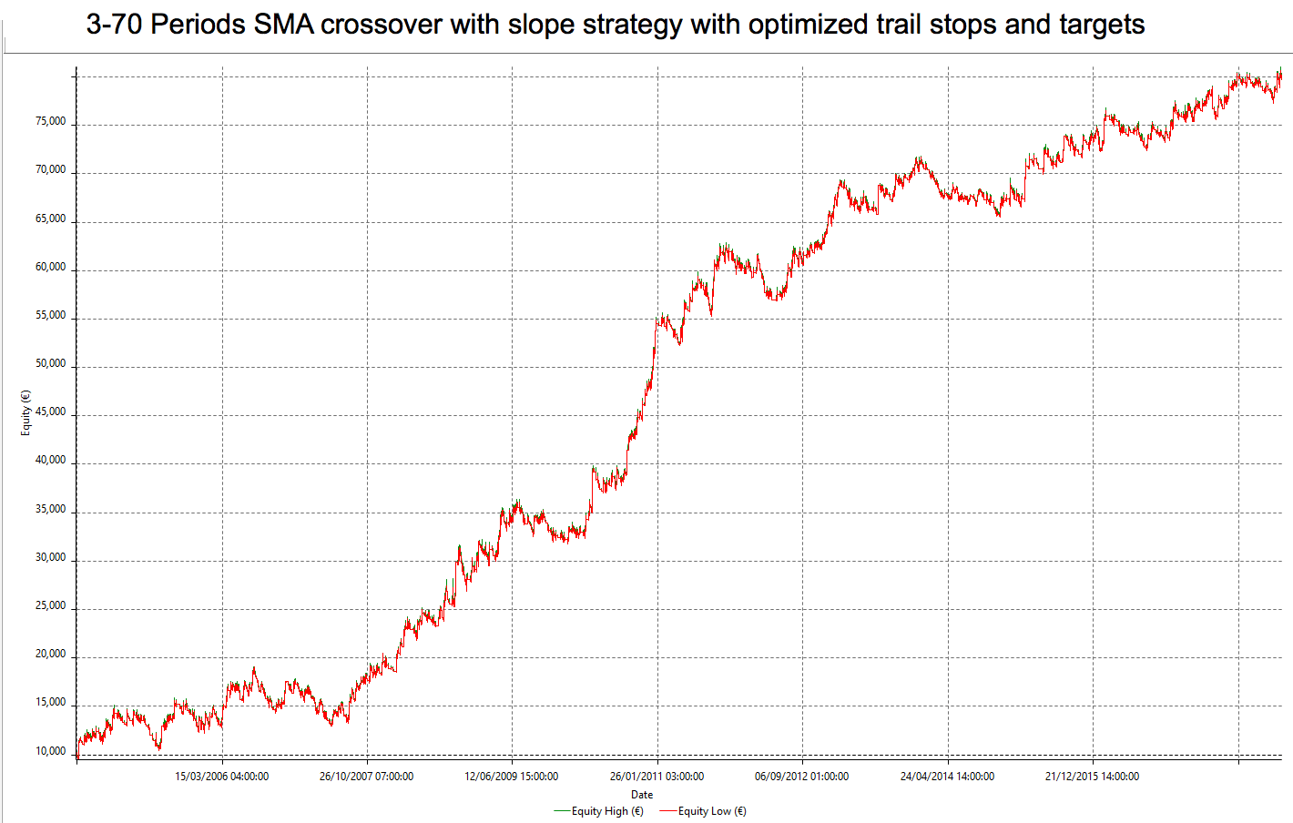
Introduction
The spread of personal computers gave investors and traders the opportunity to perform sophisticated computations in an attempt to extract information out of the naked price series. Many traders
The spread of personal computers gave investors and traders the opportunity to perform sophisticated computations in an attempt to extract information out of the naked price series. Many traders believe there’s a hidden structure in the markets, and the harder and computationally difficult the indicator is (such as ARIMA, MESA or Fourier analysis) the better. Unfortunately, until now, no computational formula reveals the secret turns of the markets, and if there is one, I don’t think the person or organisation that owns it will show it to the rest of us. But I honestly believe there’s no such formula. The era of deterministic theories of reality is gone. That is clear to me since I’ve been introduced to the quantum theory of physics. More on this: http://www.hawking.org.uk/godel-and-the-end-of-physics.html
But that doesn’t mean technical studies are worthless. There are well known and relatively simple indicators designed to give us information difficult to see or detect by just looking at the price movement, or at least to help us confirm the pattern that price is shaping.
In this article, we’ll study Welles Wilder’s DMI/ADX study
This study came to answer two questions by trend followers: Is there a trend or not? And how strong is it? And these issues aren’t trivial. Trend following traders looks to enter as soon as possible on a trend, usually on breakouts. But, if the market isn’t trending, they enter on a breakout and watch their initial profit become a loss as the breakout fails.
The proper interpretation of ADX help traders to avoid potential losses due to false breakouts, helping them focus on trendy markets, and apply other trading tactics when the signal shows the market isn’t trending.
Directional Movement was developed by J. Welles Wilder Jr, and described in his book New Concepts in Technical Trading System (1968). The DMI indicator is a very useful technical study that shows the market direction. One DMI derivation, the ADX, allows us to quantify the strength of a trend.
The directional movement DI is based on the idea that if the trend is up, the current bar’s high should be above the previous bar high. Conversely, if the trend is down then the current bar’s low should be lower than on the former bar. The difference between the current high and the previous one yields +DI, while, the difference between the current low and the previous one results in –DI. Inside bars are ignored.
Computation of the DMI
DI, the directional indicator, is computed by dividing DM by the True Range (TR).
DI = DM / TR
TR, the true range is the biggest of these three quantities:
High – low
High – close
Close-low
The resulting DI calculation may be positive or negative. If positive (+DI), it’s the percentage of the current bar’s true range that’s up. If negative (-DI), it’s the percentage that’s down for that bar.
The DI’s are averaged over a period. Mr. Wilder suggests 14 bars.
The calculation for 14 bars is:
+DI14 = DM14 / TR14
Where DM14 and TR14 are the averages of those quantities over a 14 bar period.
ADX is derived from +DI and +DI, using the following steps:
DIdiff = | [(+DI) – (-DI)] |
DIsum = [(+DI) + (-DI)]
DX = 100 x DIdiff / DIsum
The 100 scales the DX values between 0 and 100.
DX is too wild to be used directly, so we compute a moving average of DX and call it Average Directional Indicator, ADX. Usually, the smoothing average has the same period as the one used to obtain the DI.
Another indicator may be created using a momentum-like derivation of ADX called Average Directional Movement Index Rating (ADXR)
ADXR = (ADX – ADXn) / 2
Where ADX is the value for the current bar and ADXn is the ADX for the nth bar ago.
When drawn on a chart, if +DI is above –DI, then the trend is up. The opposite situation means a downward move.
If the two lines diverge, the directional movement increases. The greater the difference, the stronger the trend.
According to Wilder, the 14-period averaging was chosen because of his idea of a half cycle. Day or swing traders may choose to modify it based on the half cycle of the time frame he is trading. For instance, LeBeau and Lucas in their book recommend 12 bar averaging on a 5-min chart.

Fig 2 shows the hourly EUR/USD and the DMI & ADX study. We observe that on the left quarter, when there’s no trend, the ADX is below 25, touching the +DI and -DI lines; and these lines themselves are crossing over each other every few bars. Then a breakout in price matches the growth of the ADX line, while +DI crosses over –DI. The ADX signal grows while the trend keeps moving up with increasing strength.
The top formation changes its character and goes down following the price until –DI crosses over +DI and, then, ADX starts growing again, while price keeps falling: A downtrend is confirmed.
The sideways channel forming a local bottom hurts the ADX again, and then the small reaction up (+DI crosses over -DI) moves it up. Then the sudden drop in 5 bars makes a slight dip but ADX is up again. Then, on a new price floor (support), ADX drops again, and so on.
It seems sluggish and untimely. Many people discard it because of that. But we must remember the ADX indicator shows only trend strength.
The DI system tracks the fight between bulls and bears. It measures the power of bulls and bears to move prices beyond the previous bar range. When +DI is above -DI it shows that bullish sentiment has dominated the market so far. -DI above +DI shows the bears are in control. Thus, following the direction of the upper line is an edge.
ADX rises when the spread between +DI and –DI grows. It shows that the market sentiment (bull or bear) of the dominant market group gains strength, so the trend is probably continuing.
ADX drops when +DI and –DI are approaching each other. This shows that the dominant group is losing strength and the health of the trend is in question.
The real value is as a filter for entries. It’s important to understand that the ADX alone doesn’t show market direction, but the strength of a trend. We should use the +DI and -DI crossovers to determine direction.
References:
Computer Analysis of the Futures Markets, Charles LeBeau and David W. Lucas.
The New Trading for a Living, Alexander Elder.
Introduction
Coming from the Latin word that defined the Roman coin denarius. Money is, in general terms, the preferred means for the exchange (charge vs. payment) of goods and services
Introduction
Coming from the Latin word that defined the Roman coin denarius. Money is, in general terms, the preferred means for the exchange (charge vs. payment) of goods and services
Coming from the Latin word that defined the Roman coin denarius. Money is, in general terms, the preferred means for the exchange (charge vs. payment) of goods and services, likewise cancellation and/or acquisition of rights or obligations.
It can be associated with other functionalities or uses:

MONEY AS A MEDIUM OF EXCHANGE.
Money facilitates any exchange of goods and services among economic agents and reduces transaction costs. Any economic system with a high degree of specialization and division of labor uses money as a medium of exchange or payment of goods produced and services provided by different individuals or persons.
An economic system that excludes money as a medium of exchange of these transactions, involves the application of mediation type barter, time banks…
The following properties are required to achieve the present functionality:
MONEY AS A STORE OF VALUE.
To be able to recognize it as such, money must satisfy the characteristics of durability, allowing people to keep or accumulate wealth through savings.
Money brings the advantage of its liquidity, understanding this in its broadest possible terms, i.e., the temporary capacity that offers any good to be converted to money, without losing its value in commercial terms over time.
Time can affect the value of money in terms of purchasing power and its relation with market prices in its three temporalities: past, present, and future.
MONEY AS A UNIT OF ACCOUNT.
Environment-related to the setting of market prices of goods and services, as well as the control of accounts (accounting).
The monetary unit defines how to measure the expression of the value or market price. Each economic zone shall define its official monetary unit €; $; £…

MONEY CLASSIFICATION:
There are several kinds of money varying in liability and strength. When there was ample availability of metals, metal money came into existence later it was substituted by the paper money. According to the needs and availability of means, the kinds of money has changed.

COMMODITY MONEY
Commodity money is generally accepted as means of payment or exchange and is purchased or sold as an ordinary asset. Gold and silver have been the most common precious metals used as money. The value of this kind of money comes from the value of the resource used. It is only limited by the scarcity of the resource.
Some features: Durability; divisibility; transportable; homogeneity; limited offer…
Ex: gold coins, bread, metal, stones, tea, camels…
FIAT MONEY
A term used to denote a specific form of currency, not bound to any metal supporting it. A significant amount of the paper currency available all over the world is fiat money. Fiat money is backed by national governments as the recognized official medium of payment. Fiat money does not hold any inherent worth of its own, and they do not have the support from any form of reserve, as well. It is operating solely on faith, like the sterling used in Scotland. Nowadays, Fiat money is the basis of all the modern monetary systems. The real value of fiat money is determined by the market forces using demand and supply.
The fiat currency is also sanctioned by the Government for payments of taxes or other legal, financial obligations.
FIDUCIARY MONEY
Is conventionally maintained on a trust. The fiduciary normally retains the assets for a certain beneficiary, who could even be an executor of a will. Payments of fiduciary money could also be made in commodity money like gold or fiat money. Bank Notes and Checking Accounts are examples of the conventional forms of fiduciary money which, in this case, are provided by Banks.
Fiduciary money can be obtained from banks in the form of credible promises. These promises are eligible to be transferred and do perform the functions of conventional money.
The present-day world attaches higher importance to the token money whose variations are fiduciary money and fiat money, which differ significantly from commodity money.
Ex: Bank Notes, checking accounts…
COMMERCIAL BANK MONEY:
It´s possible to describe a commercial bank like an entity that essentially deals with loans and deposits from major business organizations and corporations. Are the most important components of the whole banking system.

The Central Banks and its functions
A Central Bank is a public entity, autonomous and independent of the Government, responsible for the monetary policy of a country.
There´re seven examples of important Central Banks around the world:
 Among its functions we can highlight:
Since it is responsible for Price stability, Central Banks must regulate the level of inflation controlling the money supply, through the use of monetary policy. A Central Bank performs open market transactions that either inject liquidity into the market or absorb extra funds, directly affecting the level of inflation.

Money Creation
The majority of money in the modern economy is created by commercial banks when making loans.
Money creation in practice differs from some popular misconceptions — banks do not act solely as intermediaries, lending out deposits that savers place with them, and they do not ‘multiply up’ central bank money to create new loans and deposits, either.
The amount of money created in the economy ultimately depends on the monetary policy of the central bank. In normal times, this is carried out by setting interest rates. The central bank can also affect the amount of money directly through purchasing assets or ‘Quantitative Easing.’
Quantitative Easing (QE) is an unconventional form of monetary policy where a Central Bank creates new money electronically to buy financial assets, like government bonds. This process aims to directly increase private sector spending in the economy and return inflation to target.
The aim of quantitative easing is to encourage spending, keeping inflation on track to meet the Government’s inflation target.
QE works, i.e., when we buy gilts, it pushes up their price and so reduces the yield (the return) that investors make when they buy gilts. This encourages investors to buy other assets with higher yields instead, such as corporate bonds and shares. As more of these assets are bought, their prices rise, pushing down borrowing costs for businesses, encouraging them to spend and invest more. We also buy a smaller amount of corporate bonds, which makes it easier for companies to raise money which they can then invest in their business.
Money creation processes by the aggregate banking sector making additional loans

 Limits to broad money creation
That occurs both directly, through influencing the loan rates charged by banks, but also indirectly through the overall effect of monetary policy on economic activity in the economy. As a result, the Central Bank is able to ensure that money growth is consistent with its objective of low and stable inflation.

Money Offer
The total amount of existing money, also called money supply, in an economy consists of cash in the hands of the public and the deposits held in the banks.
That amount of money grows or decreases as a result of bank credit and preference for the public’s liquidity, which together determine the value of the monetary multiplier.
The money supply, M, is, therefore, the result of the expansion of the base money, M0, due to the effect of the monetary multiplier m:
 In the money multiplier process, the key is in a very important proportion: the ratio between the reserves of the banks (they correspond to their deposits in the central bank) and the deposits of the public in the banks plus other liabilities.
Banks want to keep that ratio at a certain level, partly to have liquidity with which to deal with withdrawals of funds from their customers and operations with other banks, but, above all, because their central bank, usually, requires them to maintain this relationship above a minimum level.
Depending on the central bank they have different names:
Therefore, banks keep a slightly higher proportion than the mandatory minimum, so as not to run the risk of breaking that coefficient. Although, they are not interested in keeping a liquidity level too high because it would mean a loss of return that’s obtainable if they’re able to spend that excess liquidity to buy profitable assets.
Then, when the volume of reserves of banks increases above the mandatory minimum ratio, bank entities may grant credit to the private sector and the public sector. The opposite occurs when their volume of reserves is decreased.
An example to clarify this issue:
Let’s assume that the proportion desired by the Central Bank in a certain country is 2%; that is, for every 100 monetary units in deposits, banks need to hold two 2 units in liquid assets.
Imagine that yesterday all banks fulfilled that proportion, and, today, the volume of liquid assets on a certain bank has increased by 100 monetary units. Now, its coefficient is higher than the 2% desired, therefore, the bank will be interested in placing all or part of that surplus, awarding, for example, a credit to the private sector.
How will the maximum amount be known? If the numerator has increased by 100 monetary units and the quotient has to remain 2%, the denominator is allowed an expansion of up to 5,000 monetary units. The process of creating money and the process of creating credit have been launched, the final result of which is a high multiple of the initial operation.
We should understand that the amount of money in circulation varies at every moment, due to the thousands of simultaneous operations of creation, and destruction. It is interesting to realize that Central Banks control this creation process, and for this purpose, it needs a mechanism to increase or reduce the reserve account of the banks and a mechanism to regulate the creation of credit when the reserves grow, as previously commented. It is here when the so-called Monetary Policy is applied.

Each central bank has its own objectives. As is the case of the ECB, whose sole objective is price stability through a low and steady inflation rate of less than or equal to 2% per annum. On the contrary, the FED pursues two objectives: price stability without a quantified inflation level, and maximizing employment, together with the sustainability of long-term interest rates.

The implementation of the monetary policy requires the use of one or several instruments for the creation and destruction of reserves, thus, establishing the initiation of a process of creation or destruction of credit and money.
Although they manage a wide set of tools, they can be summarized into three:

 Interest rate
The interest rate is a variable that is present in almost all decisions of households, companies, financial entities and Governments. These decisions refer to actions or consequences that take place at different times of time and therefore, the interest rate represents the price of time. We could interpret it as the prize that is demanded to delay the enjoyment of something from today until tomorrow or the premium that you have to pay to advance that enjoyment from tomorrow to today.
Although there are many types of interest, let’s focus on interest rates of assets and liabilities and financial operations; so we would be dealing with the returns obtained when lending or placing wealth in a financial asset or the cost of Debt.
As already mentioned, central banks usually use two instruments to increase or decrease the circulation of liquid assets or reserves held by banks:
Central banks usually manage these instruments through a very short-term interest rate. Following the examples of the previous central banks, it is known that the ECB periodically announces an interest rate of the main financing operations that serves as a guide to the banks to the banks for the weekly credit auctions. The extent of that interest rate and its expected future changes will be a useful indicator of the expansive or contractive nature of monetary policy. An increase in that interest rate is indicative of a tightening of monetary policy, that is, a liquidity contraction and a higher cost of central bank credit, as well.

In the FED’s case, this decision sets the federal funds rate, indicating the interest rate at which it is willing to buy public debt to the banks to provide them with liquidity or, to sell it, thus, withdrawing liquidity. Therefore, that rate and its expected or announced changes will also imply changes in the sign of monetary policy.
However, the central bank controls the short-term interest rate, but families, companies, and Governments are mainly affected by the longer-term rates. This means that monetary policy has a limited, but real, effectiveness on financing conditions.
Therefore, a better understanding of the role of monetary policy in setting interest rates establishes:
Central Banks, at best, can only control nominal rates, because the expected rate of inflation will depend on the expectations of economic agents.
In a simplified way, the likely evolution of the relationship between short and long-term types in a country is as follows:
If we take as starting base a situation of a balanced performance of the economic activity, with normal market returns and subsequently, the economic activity accelerates, along with inflation expectations, its likely outcome will be a rise of the long-term interest rates.
Under these conditions, it is likely that the central bank decides to practice a restrictive monetary policy, and therefore, a rise in the interest rates in a very short time.
This monetary policy will end up moderating production and prices. As the markets anticipate this result, the long-term rates will fall again and the central bank will be able to reduce the restrictive nature of its monetary policy by returning to equilibrium.

 Inflation shows the upward or downward movements of thousands of prices, which implies the difficulty in identifying the continuous and sustained changes in the set.
However, the accuracy shown is relevant because a price variation may arise from many possible causes. In the same fashion, it happens on the movements and one-time changes in many prices, and, also, on the seasonal changes. But beware: a continued and sustained rise in the overall level of prices will not happen without any visible cause.
Who is worried about inflation?
Why?
If we take supply and demand as our base assumption, many possible causes can be identified, some on the demand side, such as the increase in consumer income and others on the supply side, such as an increase in the productive factors or the tax levied on the product.
Please note that a significant rise in prices will reduce the purchasing power of money, which leads to a monetary concentration. That will, in turn, raise interest rates and slow down the growth of production and prices. However, this will not happen if the growth of money supply is accelerated, which reduces the real interest rates, and, consequently, founds the increase in aggregate demand (consumption, investment, public expenditure, exports, and imports).
Faced with this reality, the following we may state the following:
In addition, it can also be a sufficient condition for inflation since if economic agents receive more money than they need to finance their transactions, they will spend it, and in that process, they will generate an increase in the demand for goods and services and a rise in prices.

Inflation is always a monetary event caused by the excessive growth of the amount of money concerning what is necessary to finance the real growth of the economy. That explains why Central Banks are committed to controlling inflation: because they control the amount of money.
To understand the relationship between Central Banks and inflation, it should be conceded that usually, the monetary authority of a country establishes the objective of its monetary policy in terms of the desired inflation rate (∏*). This rate of inflation that is usually low, stable and positive, will be the one that the monetary authority tries to achieve in a relatively long term and in this way avoid an erratic monetary policy. Sometimes they include a goal regarding the rate of growth of the gross domestic product, trying to match the potential growth rate of the economy (y*), compatible with a complete use of resources, so that below (left) it, costs tend to be reduced by the pressure of unemployment and above (right), costs tend to increase due to over-use of resources. Therefore, observing the following table, it is understood that point A is the one desired by the monetary authority, as previously mentioned.

If the economy is at point E, the Central Bank will practice an expansive monetary policy and keep interest rates low. When approaching B, it will probably raise the interest rate, with the objective of preventing the economy from moving to the right of y* (before arriving at A) given the slowness of the effects of monetary policy.
In C the monetary policy of the Central Bank will be clearly restrictive, in an attempt to return to A.
In D, the Central Bank will be faced with several alternatives: If it pursues the objective of inflation the action will raise interest rates with the consequent accentuation of the recession. Establishing here an observation beacon for monitoring the reaction of economic agents. I.e. The fear that trade unions might push for higher wages increases the likelihood of an interest rate increase. This explains the reason for the reaction of the Central Banks to the rise in costs such as oil or ad valorem taxes even if they produce one-time price increases → The fear that that may turn into wage increases, even more so if they use automatic indexing on wages.
An inflation like C is attacked by the use of a restrictive monetary policy, and a reduction of the rate of growth in production is the first parameter to be affected, which will shift to F, and solely after a while, it will end up achieving the objective: A.
Inflation is maintained around the desired level ∏* through an expansive monetary policy but at a very moderate level, and it must be accompanied by other measures such as:

Value: To be able to add the production of heterogeneous goods and services and express them in a common monetary unit: Pound Sterling, Dollar, Euro.
Final: To avoid the problem of the double accounting of goods that become part of the production of other goods and services, such as raw materials and intermediate products. GDP equals added value.
Of Production: Not of sales.
Of goods and services: But only the remunerated ones, so leisure, study, bricolage… and the legal ones are excluded. Underground economy and the illegal activities are not included: drug trafficking …
In a country: Region or city. It will depend on what you want to cover.
During a given period: (one quarter, one year …). Transactions carried out with goods produced in the past are not included.
At market prices: (sale to the public) including net indirect taxes (VAT).
To understand GDP, it is necessary to know other concepts related to:


There are three procedures to calculate the GDP of a country:


©Forex.Academy
Introduction
In 1978, J. Welles Wilder Jr published the Relative Strength Index (RSI) in the book “New Concepts in Technical Trading Systems.” Wilder describes the RSI as “a tool which
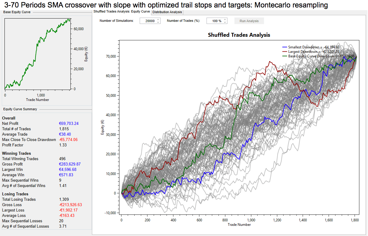
Introduction
In 1978, J. Welles Wilder Jr published the Relative Strength Index (RSI) in the book “New Concepts in Technical Trading Systems.” Wilder describes the RSI as “a tool which
In 1978, J. Welles Wilder Jr published the Relative Strength Index (RSI) in the book “New Concepts in Technical Trading Systems.” Wilder describes the RSI as “a tool which can add a new dimension to chart interpretation.” Some of these interpretations are tops and bottoms identification, divergences, failure swings, support and resistance, and chart formations.
The Relative Strength Index is probably the most popular indicator used by professional and retail traders. It’s an oscillator which moves in a range between 0 to 100. A. Elder describes the RSI as a “leading or coincident indicator – never laggard.” In this article, we will show these different ways to use the RSI.
The theory about this indicator states: “when the RSI goes above 70 or below 30, the Index will usually top or bottom out, before the real market top or bottom, providing evidence that a reversal or at least an important reaction is imminent”. Some traders have modified these levels to 80 – 20.
The basic trading idea is:
A trading system based on this interpretation is an easy way to lose money. The following example shows what I mean:

Figure 1: Tops and Bottoms signals
Source: Personal Collection
In figure 1, an example of a trading system based on Top and Bottoms is shown, with RSI levels of 30 and 70 (or 20 and 80) as entry signals. To make it short, most of the time the entry signals were false and didn’t allow catching significant trends.
Divergences are the most popular use; Wilder describes the divergence between price movement and RSI as a “very strong indication that the market turning point is imminent.” Divergence takes place when the price is increasing, and the RSI is flat or decreasing (this is known as bearish divergence); the opposite case happens when the price is decreasing, and the RSI is flat or increasing (bullish divergence).

Figure 2: Divergences
As shown in Figure 2, the divergences are a price weakening formation. That does not mean that it’s a turning point or that you should position yourself in the opposite direction.
LeBeau and Lucas describe Failure Swing as a formation “which is easier to observe in the RSI study itself than in the underlying chart.” A strong indication of market reversal occurs when the RSI climbs above the 30 level or plunges below the 70 level.

Figure 3: Failure Swing
As we can see in figure 3, the failure swing is part of the divergence concept, and it only confirms that the divergence is real. But you must pay attention and be careful with the failure swing as an entry signal because it is not a rule. The potential trade requires price-action confirmation.
The theory says that “support and resistance often show up clearly on the RSI before becoming apparent on the bar chart.” Some authors use the 50 level as a support level in a bullish trend or as resistance in a bearish trend. Hayden proposes the following rules for each trend direction:

Figure 4: Support and Resistance.
In figure 4, the RSI shows how the RSI works as support and resistance on a bearish and a bullish trend. In the bearish trend, the 60-70’s zone is acting as resistance levels and 30-20’s zone as support. In a contrarian case, during the bullish trend, 70-80’s are the resistance zone, and 40-30’s the support zone.
The RSI could display a pattern similar to those present in chart formations which may not be clear on the price chart, for example, triangles, pennants, breakouts, buy or sell points. A formation breakout indicates a move in the breakout direction.

Figure 5: Chart Formations
The most common formation is the triangle as a consolidation pattern before an explosive move. However, also is common to see false breakouts before the real move (see figure 5).
Buy Signal: When RSI breaks above its downtrend line place an order to buy above the latest price peak to catch the upside move.
Sell Signal: When RSI breaks below its uptrend line place an order to sell short below the latest price to catch a downside breakout.
We must consider that, usually, the RSI breaks its trendline one or two periods before price does. In this sense, it’s important to get a confirmation using price-action.
To summarize, the RSI is a popular indicator between professional and retail traders alike. It’s characterized by being a leading indicator. While every one of those styles (divergences, failure swing, support and resistance, and chart formations) can be used independently, that’s not a powerful tool.
A more reliable way to apply the RSI is using a mix of those methods, but the main issue here is how to trade using the RSI.
Some tips to use the RSI:

Figure 6: Trading with the RSI (*)
Source: Personal Collection

Figure 7: Trading with the RSI (*)
Source: Personal Collection
As you can see figures 6 and 7, the RSI is an indicator that does much more than an identification of overbought and oversold price levels. It helps us detecting trade opportunities, areas of movement exhaustion, confirmation of price patterns (price level failures), and chart patterns. However, RSI signals and patterns should only be used as a guide. A relationship of those signals with the price action should always be present.
(*) This is a simulated analysis and trade application.
SUGGESTED READINGS
Keywords:
Technical Indicators, RSI, Education.
©Forex.Academy
Introduction
Before proceeding to discuss forward-testing and Montecarlo permutations, we need to know the basics of the methodology and statistical foundations of evaluation and hypothesis testing. To achieve that, I’ll
Introduction
Before proceeding to discuss forward-testing and Montecarlo permutations, we need to know the basics of the methodology and statistical foundations of evaluation and hypothesis testing. To achieve that, I’ll
Before proceeding to discuss forward-testing and Montecarlo permutations, we need to know the basics of the methodology and statistical foundations of evaluation and hypothesis testing. To achieve that, I’ll use as a reference the excellent book Evidence-Based Technical Analysis – Applying the Scientific Method and Statistical Inference to Trading Signals, by David Aronson.
According to Dr. Aronson, traditional Technical Analysis is nowadays where medicine stood before it evolved from faith-based art into a system of knowledge based on science. His book’s central theme is that TA must grow from anecdotal and unproven evidence into rigorous observational science since the scientific method is the only rational way to extract useful information from market data.
The fundamental block of knowledge is the declarative statement, also known as a proposition or claim. A declarative statement is distinguished from others in that it exhibits a true or false value. The statement “Now it’s raining” or “the earth is round” are declarative, because we can assess if they are true or false. Statements such as “what is that?” or “buy me a sandwich!” do not hold any true or false value, so they are not declarative statements.
Regarding TA, an example of a proposition might be MA crossovers have an edge, and the goal of our work, when testing these rules, is to determine which of such statements justify our belief.
Therefore, what’s the meaning, of ” I believe I can buy K for $10 “? It means I expect to be able to buy K for $10 if I go to the market. But the command “buy me K!” or “I’m not happy with that price!” doesn’t have that property.
To conclude, we recognize any statement as a candidate for a belief if it holds something that we could expect or experience. Such a class of assertions is said to have cognitive content, something that can be known.
Sometimes, although a declarative statement seems to hold cognitive content, it does not. These pseudo-declarative statements are meaningless claims or empty propositions.
Although empty claims are not valid candidates for belief, this is not reason enough to stop people from believing them. Astrology pages are still prevalent in newspapers, and there are channels dedicated to astrological predictions, and pseudo-curators claim they can cure cancer by imposing their hands.
A way to detect if a statement has cognitive content is the discernible-difference test: Propositions with cognitive content make claims that are true or false, if it holds cognitive content then we can discern a difference between those two states, meaning that its truth-state is distinguishable from its false one. Testing a claim based on the discernible difference is central to the scientific method.
The best definition comes from David Aronson: Knowledge can be defined as a justified true belief. Hence, for a declarative statement to qualify as knowledge, not only must it be a candidate for belief, because it has cognitive content, but it must meet two other conditions as well. First, it must be true (or probably true). Second, the statement must be accepted with justification. A belief is justified when it is based on sound inferences from solid evidence.

Some statements seem to be true, but they aren’t. An example is ancient people believing the Sun was orbiting the earth. It seems true, but we know it’s false. These people weren’t in possession of knowledge. Let’s suppose there was a person at that time that believed the appearance of the Sun by the east every morning was due to the rotation of the Earth. Even if his belief was true he had no evidence to support that theory, so we cannot say this person had knowledge. We can call this kind of belief false knowledge because it is erroneous or there is no evidence to support it.
Finally, even when we have evidence to infer that something is knowledge, that’s not enough guarantee that we really know. Uncertainty is inherent in the scientific method, but knowledge improves with time when using the scientific method.
There are two kinds of technical analysis (TA). Subjective TA and objective TA.
Subjective TA is a not-well-defined analytical method because it cannot be expressed as a set of precise rules. Therefore, it requires the interpretation of the analyst. As a consequence, it is impossible to confirm or deny its efficacy.
Objective TA is well-defined and repeatable. That allows to implement it as a computer algorithm and back-test it using historical data.
It’s evident that a subjective TA method cannot be called knowledge since no one can reproduce it and there is no way that, even the same person, was capable of producing the same results on the same dataset. These subjective TA methods are problematic in that they present the illusion of true cognitive content, but, really, they are meaningless claims.
Objective TA can deliver erroneous beliefs, but they come from a different path. The fact that it has been profitable on a back-test is not enough to guarantee its validity. Success on a back-test is necessary but not sufficient. Past performance could be the result of overfitting or luck.
The scientific method is the most valuable knowledge the West has given to the world, according to C. Van Doren because it’s a set of procedures to acquire new knowledge. The rigorous rules of the scientific method protect us from the weaknesses of our minds. Informal observation and inference from inadequate or insufficient data are likely to fail with complex or noisy data.
Traditional TA is one of the branches of our practice that has not been applied using scientific methods. There is no surprise that many TA practitioners are against using scientific methods and say that objective TA does not capture the subtleties of all parameters involved; that only a human brain can do that. That happened in medicine as well, and when alchemy developed into chemistry.
Science aims for the highest objectivity by restricting itself solely to demonstrable facts about the world, although we understand that wholly objective knowledge is never feasible. That eliminates subjective opinions that are inherently personal.
Therefore, scientific knowledge must be open to verification by others, and it must be public to promote the maximum agreement between independent observers.
Observations must be translated into numbers to be analyzed rigorously. Quantification allows the application of robust statistical methods. Quantification is the best way to ensure objectivity and maximize its potential to be tested.
One of the goals of a scientific theory is to discover rules that predict new facts, and an explanation for past observations. Explanatory theories go one step beyond predictive theories in that they tell us why A follows B instead of just saying that it does.
The most important type of scientific law is function. It describes a set of observations in the form of an equation, such as:
Once we find a functional description, we can predict future events of Y by introducing known values to the function f(). Functions can be found by two methods: Deduced by analytical theories or estimated from historical data by fitting a function, regression analysis for example. TA falls into this second category.
Science relies on logic and empirical evidence to arrive at conclusions, as opposed to the informal reasoning that tends to find support in authority and tradition.
The fundamental principle of formal logic is the rule of consistency. It is backed by two laws: The law of excluded middle and the law of noncontradiction.
“The law of the excluded middle requires that a thing must either possess or lack a given attribute. There is no middle alternative. Or said differently, the middle ground is excluded.” {1}
“Closely related to the law of the excluded middle is the law of noncontradiction. It tells us that a thing cannot both be and not be at the same time.”{2}
A Proposition is a declarative statement that may be true or false
An Argument is a set of propositions, one of which is the conclusion, derived from the previous propositions, called premises.
A logical inference has two forms: deduction and induction.
“A deductive argument is one whose premises are claimed to provide conclusive, irrefutable evidence for the truth of its conclusion” (Aronson).
A usual form of deductive argument is the categorical syllogism, credited to Aristotle (4th century B.C.), formed by two strong syllogisms called premises and one syllogism called conclusion. Example:
Premise 1: All mammals have warm blood
Premise 2: A dog is a mammal
Conclusion: A dog has warm blood
The general form of a categorical syllogism is:
Premise 1: All members of A are members of B
Premise 2: C is a member of A
Conclusion: C is a member of B
Deductive logic is appealing because of the certainty of the conclusion. But this only happens if the premises that are the basis of the conclusion are true and expressed in a valid form. Truth and false are properties of the propositions. Validity defines the correctness of the logical inference linking premises with the conclusion. We can demonstrate its validity using diagrams called Euler circles.

Another form of deductive argument, and of crucial importance to scientific reasoning, is the conditional syllogism, which is the basis for the discovery of new knowledge. It’s also composed of three propositions, two premises, the first one being a conditional proposition and a conclusion.
A conditional proposition is a composite statement that mixes two propositions using the words if and then. The general form is:
if(antecedent clause), then (consequent clause),
for example
if it is a mammal, then it has warm blood
If this TA rule is predictive, then its back-tested return will be positive
The second premise is a premise that affirms or denies the truth of either the antecedent or the consequent clause if the first proposition. For example, it could state:
It is a mammal
It is not a mammal
It has warm blood
It does not have warm blood
The conclusion of the conditional syllogism affirms or denies the truth of the remaining clause. As an example, let’s see the complete syllogism:
if it is a mammal, then it has warm blood
It is a mammal (validates the truth of the antecedent)
Therefore, it has warm blood (establishes the truth of the consequent)
Affirming the antecedent:
Premise 1: If A is true, then B is true
Premise 2: A is true
Valid Conclusion: Therefore, B is true
Denying the consequent:
Premise 1: If A is true, then B is true
Premise 2: B is not true
Valid Conclusion: Therefore, A is not true
This is the form that uses science to prove that a hypothesis is false. If we can prove that a hypothesis is false, we can indirectly prove that some other is true. This is the way to acquire new knowledge that we wish to establish as true. For example, that a TA signal is more predictive than a random entry.
People using informal logic tend to commit two errors: Affirming the consequent and denying the antecedent. An example of affirming the consequent is:
If it is a mammal, it has warm blood
It has warm blood
Therefore it is a mammal
The fact that the animal has warm blood it doesn’t mean it’s a mammal. This fallacy is common in TA. Let’s see an example:
If this TA strategy has predictive power, then it should be profitable in a back-test
the back-test is profitable
Invalid conclusion: the TA strategy has predictive power.
The other form of invalid conditional syllogism is denying the antecedent
If it is a mammal, it has warm blood
It’s not a mammal
Therefore, it does not have warm blood
Even in the absence of complete information, a conditional syllogism’s conclusion may enhance our knowledge about A or B:
If A is true, then B is true,
B is true
Therefore, A becomes more plausible
The evidence does not prove A to be true, but verification of some of its consequences gives us more confidence that A is true.
A weak form of reasoning using the same strong premise is:
If A is true, then B is true,
A is false
Therefore, B becomes less plausible
B is not proven false, but one of the reasons for it being true has been discarded.
Finally, a plausible reasoning is even weaker:
If A is true, then B becomes more plausible
B is true
therefore, A becomes more plausible.
In his book Probability theory, the logic of science, E.T. Jaynes presents a practical case:
“Suppose some dark night a policeman walks down a street, apparently deserted. Suddenly he hears a burglar alarm, looks across the street, and sees a jewelry store with a broken window. Then a gentleman wearing a mask comes crawling out through the broken window, carrying a bag which turns out to be full of expensive jewelry. The policeman doesn’t hesitate at all in deciding that this gentleman is dishonest.”
What’s the policeman’s reasoning process to deduct the man with a mask was a burglar? There might be a totally innocent explanation for this situation: The gentleman with the mask was the owner of the jewelry, coming from a masquerade party and while walking near his store a truck accidentally throws a big stone that broke the jewelry’s window. In the end, he was protecting his merchandise.
So why the policeman’s actions seem right? It is so because the probability of this explanation to be true is quite low. If the policeman had been experiencing this kind of situation often because there were a lot of trucks that usually throw stones at jewelry’s windows while its owner comes from masquerade parties the policeman would soon stop worrying when observing people with masks getting out with a bag full of jewels.
Therefore, our reasoning depends very much on prior information.
Induction tries to extract knowledge about the world by going beyond the knowledge contained in the premises. The new knowledge comes at the price of it being uncertain. Wikipedia philosophical definition is quite good: “the premises of an inductive logical argument indicate some degree of support (inductive probability) for the conclusion but do not entail it; that is, they suggest truth but do not ensure it. “
Inductive logic goes in the opposite direction of deductive logic. Deductive starts from general facts and concludes about a particular fact. Inductive starts from a sample of particular examples to reach a conclusion
As an example of a deductive argument:
All known life on earth depends on liquid water to exist
Therefore, it is highly probable that all biological life in the universe depends on liquid water to exist
Generalizations need not be universal. We may say as well:
X percent of A’s are B’s
Or
X Percent of B’s hold attribute A
Or
B’s hold attribute A with probability X
Unlike deductive logic, inductive logic allows for the conclusion to be false, even when the premises are true. Instead of being true or false, inductive arguments are strong or weak, with describes how likely the conclusion is right.
Inductive logic is also known as hypothesis construction because it allows us to make conclusions based on current knowledge and further predictions.
One common form of induction is based in enumeration. It starts from a premise that enumerates the evidence contained in a set of observations and a conclusion predicting the properties of observations outside the known set.
Premise: This TA rule gave 500 buy signals over a 5-year period using hourly charts, and in 300 of them the market moved markedly higher over the next 20 bars.
Conclusion: In future appearances of this TA signal there is a 60% chance that the market moves higher along the first 20 hours.
The strength or weakness of the conclusion is enhanced or weakened by the quantity and the quality of the evidence shown by the premise.
Supposing we have only ten samples with a 60% success rate the evidence on the goodness of the signal is quite poor. In that case, further evidence may differ greatly from the 60% probability in one way or another.
The quality of the evidence is also important. Some methods are better than others. The gold standard to gather evidence is the controlled experiment with all its parameters held constant, except the one subject to test. TA does not permit that kind of test, but some methods are better than others, and we should be especially careful to avoid systematic errors such as data mining bias and confirmation bias.
The availability bias causes people to depend primarily upon information that’s easily accessible to them. As an example, when asked people to signal the importance of a list of facts, they rank based on the recent news by newspapers or by their personal beliefs or experiences, disregarding less obvious evidence.
The confirmation bias is the natural inclination to seek confirmatory rather than denial evidence about their beliefs. For example, people tend to seek corroborative evidence that some TA signal is predictive, rather than disprove it.
The predictable world bias describes the tendency to perceive order where there is just randomness. Gamblers and traders find patterns where there is none, and they believe they can predict outcomes from past data.
The law of small numbers bias tends to assign a predicting value to what essentially is random noise caused by a short streak of good or bad luck. For example, when a trader has five straight wins thinks his system is excellent attributing to the system what might have been just a very lucky winning streak.
The data mining bias is the result of extensive searching for patterns on a historical database using excessive parameters or continually improving the parameter mix until we find a good result.
Sample selection bias happens when available data is not representative of the whole possible scenarios. For example, we test a TA strategy for the last five years of historical data, but it happens that during this time that market was trending up, so the strategy is not representative in downtrends.
David Hume, in his work Treatise on Human Nature, defined the problem with induction: how to distinguish true knowledge from inferior forms of wisdom such as opinions.
Before Hume, there was a consensus that the difference was related to the quality of the method employed. Hume said that the belief that A causes B or is correlated to B, just because A preceded B, was a habit of the mind. He said that no amount of observed evidence was satisfactory, and there was no rule to tell us then we have evidence enough.
Supporters of induction claimed that generalizations coming from induction were correct in a probabilistic way. However, critics said that that justification was flawed. The probability that A predicts B is equal to the number of times that A is followed by B, divided by the total number of samples, but, because an infinite number of cases will happen in the future, the result is zero no matter what the number of past observations.
It took more than two hundred years to understand the paradox between Hume’s critique and the accumulation of scientific discoveries. William Whewell was the first to understand the role of induction in the formulation of hypothesis. He said that scientific discovery starts with an inductive guess, but then it’s followed by deduction. After a hypothesis has been induced, predictions are deduced in the form:
If the hypothesis is true, then specific future observed events would occur.
The hypothesis is antecedent clause, and the prediction is the consequence clause in a deductive syllogism:
If A predicts B then future A events will be followed by B events.
When there is a cause-effect between A and B the following proposition is used:
If A causes B then if A is removed B should not happen.
Therefore, if B does not follow future observations of A, then the hypothesis is proven false by the valid deductive “falsification” of the consequent (B).
If A, then B
Not B
Valid conclusion: therefore, Not A
But if future appearances of B follow observations of A, the hypothesis IS NOT proven true, because we have to remember that affirming the consequent is not valid deductive form:
If A, then B
B
Not Valid: therefore X
Karl Popper extended the Whewell’s insight and redefined the logic of scientific discovery. Popper’s central allegation was that scientific studies were unable to confirm a hypothesis. Rather, scientific efforts were limited to identify which hypothesis was false.
Popper’s method of falsification goes against common sense, which favors confirmatory evidence. He argued that the absence of required evidence is sufficient to establish that a hypothesis is false, but the appearance of the expected evidence is not enough to determine its truth.
One implication of Popper’s method of falsification is that scientific knowledge is provisional. Every currently accepted theory may be replaced in the future by a more correct one. The net result is a body of knowledge on continuous improvement, building upon prior successful theories, and discarding wrong ideas.
Another consequence of Popper’s method is that science must limit itself to a testable hypothesis: propositions that generate predictions on events not yet uncovered (past or future).
A major consequence of Karl Popper’s method is that it solved a fundamental problem in the philosophy o science: Differentiating between science and non-science: Science is limited to those propositions that make predictions that can be refuted using empirical evidence.
A hypothesis is informative if it makes testable predictions, with the possibility that they can be found false. Therefore, the information content of a hypothesis is linked to its falsifiability.
A high information-content hypothesis makes precise and high quantity predictions. Then, it offers ample opportunities to be falsified. A low information-content hypothesis makes fewer and less accurate predictions. Therefore it is more difficult to falsify.
The hypothetico-deductive model also called the H-D method is a proposed procedure for the construction of a scientific theory. Dutch physicist Christiaan Huygens (1629-95) introduced the original version.
In the next part, we will examine the basics of statistical analysis and hypothesis testing. Both needed to continue our path to do proper trading system testing and validation.
References:
Evidence-based Technical Analysis, David Aronson
Probability theory, the logic of Science, E.T. Jaynes
Wikipedia searches on inductive and deductive logic
Encyclopaedia Britannica: https://www.britannica.com/science/hypothetico-deductive-method
Abstract
The economic cycles are one essential topic studied by the economy. There is a wide variety of literature that mentions the fluctuations and long-term trends of economies. But

Abstract
The economic cycles are one essential topic studied by the economy. There is a wide variety of literature that mentions the fluctuations and long-term trends of economies. But
The economic cycles are one essential topic studied by the economy. There is a wide variety of literature that mentions the fluctuations and long-term trends of economies. But behind these cycles and trends, there are variables that explain why the economy behaves in that way and are also affected by the state of the economy. These variables are the level of employment in an economy and access to credit by companies and individuals. When an economy is slowed, the level of unemployment increases and access to credit is restricted due to higher provisions of the banks due to a higher risk of default. It is important to analyze how these variables are found to examine which economic cycle this country is.
Some variables may be magnified or affected by economic cycles, a topic analyzed in the article Cycles and Economic Oscillations. Two of the variables that will be analyzed are employment and the financial sector. If it is possible to understand how these variables behave in the business cycle of the economy, it will be possible to understand the mechanisms of propagation of shocks. In the case of the labor market when presenting certain rigidities, it does not react immediately to changes in the economic cycle; on the contrary, it takes time to balance. There are several explanations of why real wages can be rigid.
The first theory that tries to explain why wages are rigid is the existence of long-term contracts between workers and companies. Long-term contracts provide insurance and specific parameters that must be respected by both parties so that wages can be stable over time regardless of the labor market situation. Another theory highlights the role of unions which try to ensure the employment situation of their members and the actions taken for this can generate rigidities. The last theory that deals with the rigidities of the labor market are efficiency wages. The more a person’s salary is, the more incentives they will have to develop their work better.
But efficiency wages do not explain well why wages should be rigid since companies can in some cases verify the efficiency of their workers and, accordingly, set wages. In addition, there are currently performance bonds that serve to incentivize their workers. Workers make further efforts when economic cycles are in a depression or recession phase, since unemployment increases in these cycles, which makes it riskier to lose their jobs because it will be harder to find work. Therefore, salaries will be increased when there are better employment rates because there is more incentive for workers to perform well.
The frictions of the labor market, although they generate that there is an uncoupling between the economic cycle and the labor market, also reflect the situation in which the economy finds itself because the variables of the labor market present fluctuations like the economy. Also, these rigidities generate persistence in some variables such as wages and the unemployment rate which implies that when setting monetary and fiscal policies it is necessary to keep in mind that the variables do not respond instantaneously but rather adapt slowly due to the persistence in shocks.
The difficulties of the salary to adjust to full employment and the speed with which the long-term employment flows are adjusted contribute to understanding how the product is behaving throughout the cycles. Real rigidity also helps magnify nominal rigidities, by making companies more sensitives in their utility when there are price changes. When an economy is in cycles of depression or recession, there is evidence of increases in unemployment due to lower growth which leads to more layoffs and when people try to find new jobs offer them less salary which implies a drop in productivity.
It is because of these problems that the policies of governments and financial entities should be directed to develop financial markets better and make their access easier. If there is a financial market where companies can obtain loans for the development of their activities, the destruction of employment can be avoided, which will prevent wages from falling. The credit channels will be incentivized by monetary policies that affect the volume of loans of the banks and how this, in turn, affects the aggregate demand. That the loan channels are a variable of the monetary policy that can be used in addition to the management of the interest rate by the central bank.
If there were no distortions in financial markets, the demand for funds from companies would always be covered. Due to some regulations, credit channels are not continuously available to all businesses. The companies that are most affected by these rules and behavior of banks are medium and small companies which face higher loan costs, and it is not easy to enter the capital market because there are transaction costs to issue their shares, so they also do not have access to this means of financing. In the following graph, you can see the market capitalization of several countries.

Graph 31. Market Capitalization of listed domestic companies. Data taken from the World Bank.
Credit channels are a mechanism used by monetary policy but also serve as a propagation of the economic cycle in the face of a shock. The primary source of transmission of business cycles in credit channels is the volume of loans issued by financial institutions. When there is less volume of loans due to provisions that banks have for bad credits granted, there are fewer resources to issue loans which affect the level of activity of an economy since investors cannot ask for as many resources as they would like.
On the contrary, when there are booms in the economies, credits increase as banks have fewer provisions for bad loans and can lend more. These correlations occur in most countries regardless of domestic production or the development of the financial system. It is important to mention that the provisions affect the profits of banks which also affects the incentives to lend during recessions where it is normal for many of their loans to be risky.
To carry out some projects, medium and small companies must finance using their resources or some specialized entities. Even the issuance of bonds is limited to these types of companies due to the transaction and valuation costs of their assets. These high costs faced by companies are due to information asymmetries where banks must invest part of their resources in research to the people they are willing to lend to. Besides, as already mentioned, the provisions are also costly for the utility of the banks, so the risk they face when they lend money is transferred to their potential clients. The following graph shows the percentage of domestic loans provided by the financial system. There is a relationship between higher development and a more developed and accessible financial sector.

Graph 32. Domestic credit provided by the financial sector. Data taken from the World Bank.
In addition, banks cannot always be monitoring if their clients are using their resources properly, which is called in the economy, moral hazard. Moral hazard exists when a person can have bad behaviors and has no consequences. In the case of banks, people can be irresponsible with money management and take excessive risks, so banks must monitor the behavior of people.
Finally, when the central bank increases its interest rates, the banks adjust the credits they grant depending on demand and how their balance is, and if there are no credit restrictions, there will be no additional effects to a rebalancing in the credit market. But if there are some restrictions in the credit market, increases in rates will cause banks to lend less, also affecting the utility of banks and ultimately also affecting domestic production and investment in the economy.
In other cases, it is possible that external phenomena have repercussions on the national banking system and generate a crisis. For example, if there is a decline concerning trade and a depreciation of the currency might be considered, this may place the economy in a worse equilibrium in which people start panicking. Therefore, this state of panic may drive people to try to get all their deposits out from the banks, generating an effect where the bank runs out of liquidity but with multiple obligations, which might force banks to bankruptcy. These bank failures may induce a financial system collapse, external financing cut, currency depreciates even more, and production enters a crisis.
In open economies, the ability of the government to rescue banks is limited to the availability of international reserves. In addition, when there is a crisis in an open economy with exchange rate parity, this crisis not only affects banks, it also affects such parity, so in some countries with this system of exchange rates a financial crisis and crisis of exchange can be generated at the same time.
In conclusion, economic cycles and their fluctuations can be magnified depending on the state in which some variables are found and their rigidities. The labor market can give clues about what the current state of the economy is like and in what stage it is. Besides, the financial sector also responds to these cycles, and there may be crises during periods of recession or depression if the regulations or the way banks act is erroneous. That is why it is important to analyze different areas of the economy to understand what cycle it is in, how mature is that trend and what are the lags that can be identified to forecast the behavior of domestic production of a country.
©Forex.Academy
Abstract
Some countries have valuable domestic productions such as Germany, Japan, the United States, Canada or France among others. But there is another group of countries that are representative
Abstract
Some countries have valuable domestic productions such as Germany, Japan, the United States, Canada or France among others. But there is another group of countries that are representative
Some countries have valuable domestic productions such as Germany, Japan, the United States, Canada or France among others. But there is another group of countries that are representative and are called emerging economies. This group of countries are those that grow more than the average but that their level of nominal and per capita internal production does not reach that of the developed countries. Although they are not considered developed countries, they are important countries given the size of their market, and their progress in economic and social matters. Examples of these are countries such as India and Brazil. That is why, for the world economy to grow in general, it is important that the emerging countries do well.
Just as there are countries that largely determine the behavior of most of the world’s economies such as the United States and China there is another group of economies that are important because of their growth potential, such as emerging economies. Emerging markets are countries that have made steady progress towards the development and growth of developed countries as can be seen in some indicators of social development, capital markets and clear laws and regulations on transactions. Emerging markets are not as advanced as developed countries in economic and social indicators, but they maintain more developed economies and legal structures than other countries that are lagging in terms of development.
Emerging market countries generally do not have the levels of efficiency in the production of goods and services that developing countries have mainly. Another difference is the regulatory framework of the markets that also explain some of these inefficiencies since the legal framework in some countries is not well established so there is some distrust on the part of investors when they are going to invest in a country of this group.
But the positive aspect of the emerging countries is that because of this progress faster than the developed countries, the returns on investments are in most cases higher. This faster growth is because there is a greater field of improvement in these economies because in many cases there are nascent industries or markets that have not yet been fully developed, making it easier for these countries to grow faster than developed countries when the inefficiencies are solved.
Something that is always linked to the rates of return on investments is the risk that investments face. These risks are linked to political instability, problems or delays with the local infrastructure, the volatility of the local currency or liquidity problems which represents a risk for the investments since when there is little liquidity in a market it is difficult to get returns from the investments due to the little demand.
A problem to identify countries that are classified as emerging is that there is no unanimity in the classifications since some banks have identified certain countries as emerging while there the international monetary fund has another list of countries which makes it difficult to know which are the countries in this category to follow them up. The countries most agents consider as emerging are Brazil, Chile, China, Colombia, Hungary, Indonesia, India, Malaysia, Mexico, Peru, Russia, South Africa, Thailand, and Turkey.
As mentioned in the article China and its economic predominance China has grown more than the other emerging countries so it is expected that China will soon enter the group of developed countries due to the surprising rates to which it has been growing in the last decades. Even with the change of economic model China will continue to grow at high rates and will continue to achieve social achievements. Each analyst agent has the authority to enter the level of emerging markets to any country, as well as to lower their rating to countries on the border.
The main databases that analyze emerging markets consider annually how is the environment to do business in each country and show the positive and negative aspects in the main areas in terms of infrastructure and logistics. In recent years since the global recession of 2007, there has been great volatility which has led some developed countries to see their rating downgraded as Greece, a country that has had major economic problems in the last decade.
Emerging markets, although they are sensitive to the low growth of powers and trading partners such as the United States, China, Japan, and some European countries, also have attractive and large markets for investors, which means that emerging countries are also considered engines. of the world economy.
The indexes that measure the countries that should be in the emerging category measure:
As mentioned earlier, the last few years have been years of low growth for emerging countries due to the global situation where raw materials saw their price fall, which affected the income of some emerging countries. But this low growth is general and has spread to most countries, which is explained by such a globalized economy where if there is a group of countries that stop growing or enter recession like Brazil they generate a problem in countries that are business partners as they stop consuming and ends up affecting the exports of several countries.
Until 2016, growth has been stagnating in emerging countries and some of the reasons for this are the slowdown in China which affects the price of raw materials, the instability of oil prices and the symptoms of an economy weakened in the United States, where a business cycle is observed to be terminated. Some analysts see China as one of the leaders of this group so if this country stops growing at the rates it was used to, it will generate a big impact on emerging countries’ indicators.
The other two important countries in the emerging countries are the United Arab Emirates and India which had the highest growth in 2015 and has had several reforms to improve business rules and has a market of great potential due to its size. As for Latin America in the last decade, it has offered opportunities to investors thanks to good rates of growth and political and social stability.
Since 2016, Brazil, which was among the five most important countries in emerging markets, stopped being due to the recession in which it started generated by corruption factors and reductions in the prices of raw materials. But the problems of corruption are a widespread problem throughout the region which added to the crisis of commodity prices since 2014, poverty and mismanagement of the economy have caused high growth rates that had at the beginning of the century no longer the same.
Another country that is important among the emerging countries is Mexico, a country that has managed to stand out above most of the countries in Latin America thanks to its large amount of exports and an attractive exchange rate that encourages exports even more. Mexico has a developed manufacturing sector that supplies the United States market. In addition to its manufacturing sector, it has other developed industries that are competitive thanks to low production costs where labor is almost as competitive in terms of costs to Chinese labor. Thanks to the development of its industries, Mexico has managed to develop a good infrastructure network such as railroads that allow transporting the merchandise without problems and in a short time.
Thanks to these advances in emerging markets, the global situation has changed, and the poverty rate has been greatly reduced, but a large percentage of the population still lives in poverty. It is important that emerging countries manage to follow this path of growth and progress so that the global economy advances at good rates and manages to reduce some problems such as poverty. Emerging economies are called to lead global economic growth in the coming years, but not only depends on them with an economy as globalized as we have now, because if countries like the United States and China stop growing or the emerging countries faces to Recessions, they will not be able to grow at their potential rates.
But emerging economies have everything to follow their good path and continue to grow at good rates, developing their institutions and advancing in legal aspects since their societies are established under laws that are fulfilled, the level of wealth and consumption has been raised, investment has increased in recent years, in most of the years of the last decade its economic growth is going at an excellent pace. In addition, emerging countries have higher rates of growth often give better returns on investment than other countries, but we must also be cautious because these rates of return involve greater risks than other risks that developed countries may have as political risks.
Although emerging markets are countries that grow more than the average, they have some difficulties in managing their own expansion. In some countries, policies have been erroneous to encourage the population to increase their savings rate. In terms of demographics in emerging market countries, there is a big difference with developed countries. In emerging countries, the population is younger than in the developed countries and has been growing at high rates, which in a few years, will mean that these countries will provide labor to more countries and avoid some problems when the population ages as large pension liabilities.
In the following charts you can see the population pyramids of the group of developed countries of the G7 (Canada, France, Germany, Great Britain, Italy, Japan and the United States) and countries leaders among the emerging that are green in the second graph that were carried out by a study of the BBVA Bank in the year 2013.

Graph 33. (2013, October 24). Emerging Trends in Developing Countries. Retrieved December 1, 2017, from https://www.slideshare.net/BBVAResearch/emerging-trends-in-developing-countries

Graph 34. (2017, September 20). Emerging and growth-leading economies. Retrieved December 1, 2017, from https://en.wikipedia.org/wiki/Emerging_and_growth-leading_economies

Graph 35. (2017, September 20). Emerging and growth-leading economies. Retrieved December 1, 2017, from https://en.wikipedia.org/wiki/Emerging_and_growth-leading_economies
A problem that arises with demographic explosions is the rise of inequality in the middle and lower classes. To prevent this inequality from rising when economies grow, the quality of life of the lower classes should grow at the same rate as the economy does. As previously mentioned, the economic development of the emerging countries has reduced poverty within its population, but the same has not happened with the rates of inequality which at best have remained stable.
The challenge for governments so that growth does not stagnate is to create a richer middle class that can consume more and that this could be one of the most important components in domestic production. Also, if the middle class grows, they will also use the financial sector of a country more, which will generate another engine for growth. That is why it is not good to have high rates of inequality in emerging countries because this can generate growth in the short term, but it will be a big problem in the long term.
The advantage of the emerging countries is that they start from a low base of middle and low class so that wealth can grow in great magnitude given the field of great improvement that exists in these economies. But it is not enough to encourage domestic consumption. Emerging countries should attract foreign investment to finance local projects and there should be more liquidity in the economy, which favors confidence indicators in the economy.
To attract investment, countries must open their doors to companies from all countries, establishing transparent property rights and opening capital markets to foreign investors. If the financial market adopts international standards, it will generate confidence among investors and the country’s risk premium will be reduced by making local investments more profitable because the financing costs will be reduced.
Although the population is young in emerging countries and can be the workforce used by other countries, it is important that there exist incentives in the countries to retain their skilled labor and thus benefit from these local workers. If countries have problems of employability, workers will look for other countries to work in and, in some cases, with better wages than if they decided to stay in their country of origin. So, governments must worry about creating jobs that require qualified people, which sounds logical, but it is difficult to adopt due to the immediate need of some countries to create jobs regardless of the qualifications of their workers.
In conclusion, the countries of emerging economies have a competitive advantage and it is the wide field of improvement that they have in their main indicators such as employability, inequality, foreign investment, industrial development among others, which attracts capital from all over the world thanks to their generous returns where investors expect economies to grow steadily and significantly in the coming years.
Many multinationals have been in these economies recognizing the potential of these markets that have a large size as in Brazil, China, India, and Mexico. In addition, they take advantage of some advantages such as cheaper labor than in developed countries, in addition to other factors such as natural resources that provide inputs for some industries.
The economy fluctuates in some studied cycles and it is normal that it revolves around long-term trends showing its productive capacity. It is therefore normal to see a crisis in some countries cyclically and the authorities must intervene so that crises do not become persistent. But there have been crises of great magnitude such as the crisis of the 1920s, 2000s and 2007. The latter was a financial crisis that had its causes in the measures taken by the central bank and the government to solve the stock market crisis in the United States in 2000. But it was a crisis that spread to most countries in the world due to globalization in investment, so people in all countries saw the crisis originated in the United States.
Throughout history in the economy, there have been several global crises that have emerged in different countries and each has a different explanation. This article will mention some problems that have arisen in the economies and that can still be presented in the future. The first issue to be discussed is the crisis that occurred in 2007, which originated in the United States.
The starting point to understand why occurred one of the biggest crises in history we should analyze the historical price of housing in the United States. There have only been two periods in the recent history of a drastic increase in the price of housing in the United States. The first period was in the 1940s during the Second World War and was due to the low construction activity in this period and an increase in demand when the war was over.
The second episode of a drastic price increase was the first decade of the 21st century, but this second episode cannot be compared to the phenomenon of the Second World War. Construction costs were declining, and demand grew, but not of great magnitude. In the following graph, you can see the magnitude of the increase in the prices of new homes in the United States.

Graph 19. (2011, January 22). Median and Average Sales Prices of New Homes Sold in the US 1963-2010 Monthly. Retrieved November 8, 2017, from https://commons.wikimedia.org/wiki/File:Median_and_Average_Sales_Prices_of_New_Homes_Sold_in_the_US_1963-2010_Monthly.png.
As the price growth was so fast, the prices could not sustain this trend and ended up decreasing close to 30% which led to the entire US economy collapsing along with other countries that also saw as the housing market was in imbalance. The effect on the economies was magnified because part of the income of the families came from this market since they had these investment instruments, so the price reduction ended up affecting household consumption.
To explain this crisis, we must first analyze the reason for the volatility in the price of housing. The prices increased drastically first because of very low interest rates that gave liquidity to the market, making the loans more affordable and second, due to the total euphoria of the consumers who had the belief that real estate prices would never fall. again. The nominal interest rates were low since inflation was low, so the central bank had no incentive to increase these rates and since the housing price did not directly enter the inflation indicator, it did not generate inflationary pressure.
A fact that would have prevented this housing bubble would have been to include the sale prices in the consumer price indicator and thus the FED would have had to increase the rates to control inflation since the only thing considered in the indicator of prices is the value of the leases, but these did not rise proportionally to the sale prices. Another element that fueled the bubble was the regulatory change made by banks to approve the granting of mortgage loans. The following graphs show inflation and the real interest rate of the United States during the crisis.

Graph 20. Inflation, consumer prices. Data taken from the World Bank

Graph 21. Real interest rate. Data taken from the World Bank
This regulatory change made easier to access a mortgage loan, which encouraged consumers to take loans and increased bank profits. Consequently, loans were granted to people who were likely to default on their loans. But the banks did this knowing the possible consequences because with the creation of financial instruments recently banks were able to take out new and risky loans from their balance sheets and passed them on to investors who did not know the type of mortgages they had within these financial products.
This is a problem of moral hazard since the banks were less careful in the loans they granted since in principle the risk of nonpayment was no longer theirs. When the market stopped rising, some households saw that the market price of their homes was lower than what they owed to the bank, so they stopped paying their loans and the banks began to seize the real estate, but going into loss due to the decrease in prices and the costs of having to keep a property for sale. In addition, many banks leveraged lending that is to borrowed money that was not theirs since they were indebted to other financial institutions so when people stopped paying and investors who had financial instruments some banks were insolvent.
The banks that survived the crisis remained in a weak position, so they had to take some measures such as lending less and increasing the requirements or selling liquid assets such as bonds and stocks, thus incurring losses. The result of this was the significant decrease in the loans granted which ended up having repercussions on private consumption which is the main compound of most of the economies in the world, expanding what started as a financial crisis and affected the price of the shares as panic was generated after the sale of shares by financial institutions what ballasted the values of the stock market.
The financial crisis that began in the United States spread and ended up affecting most advanced economies and emerging market countries due to trade. This is the main problem of globalization because with the opening of the markets of goods consumers spend part of their income on foreign goods and as consumption in the United States was depressed, also the demand for foreign goods was affected which ended for affecting production in the other economies, especially those that depend most on international trade. In addition, as mentioned above the financial instruments created were obtained by investors around the world, which is why it also affected the purchasing power of investors around the world.
Central banks used monetary policy to lower interest rates while government entities used fiscal policy to encourage consumption and replace private demand with public demand while consumption and investment recovered. But in some countries, the nominal interest rate was close to zero, so the banks did not have maneuver margin, so they had to wait until the fiscal policy stimulated the economy almost by itself. The only thing the central bank could do was to buy assets from banks that were weak so that the cost of lending would not rise, and they could continue giving loans for investment and consumption.
Once the crisis of 2007 is analyzed, another problem will be analyzed, such as the high debt of the countries. To understand why high and growing debts are generated, one can start from the assumption of an economy with a balanced budget. At a given time, the government decides to lower taxes by keeping public spending constant generating a budget deficit.
When a government faces a budget deficit, it can ask the central bank to finance it. In this specific case, what the government does is sell bonds to the central bank or private investors. If the government decides to reduce taxes for a certain period, to rebalance state accounts, the public sector must create a primary surplus, which can be achieved by raising taxes or reducing spending. The longer the government waits to raise taxes or the higher the real interest rate at the time of paying off debts, the higher the tax increase will have to be in the year to prevent the debt from increasing further.
Also, to pay interest on the bonds in each year that continues to have a deficit every year should have a primary surplus and thus not alter the level of existing debt. The longer a government waits to raise its taxes and create a surplus in its accounts, the stabilization will be more difficult because the tax increase will have to be much greater over time as the debt will increase. If this problem is not solved in the short term the debt will have high levels as a percentage of GDP and a debt crisis will be unleashed as interest rates increase and so will the government’s main debt, which will be a vicious cycle.
It is at this point that the idea of failing to pay the doubt to lower taxes or to increase public spending begins to seem attractive. But if this happens the government will have difficulties to finance itself in the future since the investors will not have credibility in the government and will ask for higher risk premiums within the interest rates of the bonds, so it will be a problem in the long term. In addition, this measure can affect the consumption of households by affecting their wealth as some will be holders of bonds that the government does not pay.
Many times, the correction in the debt does not arrive in time since the governments are reluctant to accept that the debt is becoming a serious problem or because there is political interest in maintaining certain policies such as tax reduction to win elections and not affect economic groups. important in the voting. In summary, governments can take three measures to correct deficits, the first is to increase taxes or reduce costs, the second is to finance through the central bank or stop paying the debt, but all these measures have their negative effects on both the balance of the government as in the consumers.
The last problem of the current economy that will be dealt with in the article will be high inflation. In the past, when the authorities could determine the monetary policy of central banks, this authority was used to print money to finance their spending. When the authorities did this, higher inflations were generated that ended up affecting consumers and investors through very high inflation rates. Currently what the rulers can do is request cooperation with the central bank so that the government issues bonds and the bank buy them with new money, that is, printing banknotes by the central bank which will have the same effect as if the government issue new money.
The phenomenon explained above is called monetizing the debt and it is not the main policy used by the government and the central bank, but there is a possibility that can occur. If this type of financing is used, hyperinflations that are large increases in inflation could be generated and become a repetitive one since inflation is indexed in certain goods of the economy, so if inflation is very high in a period, is likely to be in the next period very high
Hyperinflation would be generated if the nominal amount of money increased and is maintained indefinitely causing an increase in effective and expected inflation. When inflation overflows the fiscal deficit will also be affected since the purchasing power of people will be reduced and the collection of taxes from the government will take more time. In addition, taxes are collected on past nominal income and their real value decreases with inflation over time.
To curb hyperinflation governments must have a stabilization program that contains a fiscal reform and carries out a credible reduction of the budget deficit. Also, show and promise that the central bank will not monetize more the public debt of the state. If the problem of inflation is very large, a drastic measure that some countries have taken is to take the dollar as the national currency to reflect the fact that it does not have control over monetary policy.
©Forex.Academy
The central bank and the government have tools to accelerate the monetary policies or contract the economy such as the interest rate, public spending, the amount of money in the economy among others. But when an economy is exposed to international trade some factors can have undesirable effects on the local economy. That is why when the authorities are going to intervene in the economy they not only think about local theoretical models, they also must think about how these measures will affect trade with other countries and how the trade balance of the country will turn out. Not only will the trade balance end up affected, but also the exchange rates with other currencies and therefore the purchasing power of people, so it is essential to analyze the effects in an open economy of economic intervention.
With globalization, economies face various challenges as seen in the article Globalization and its risks. One of the most important decisions faced by central banks and authorities is the determination of the exchange rate and the economic policy that each country will take depending on the objectives pursued by the government and the central bank. Economies that are exposed to international trade and thus to globalization are called open economies. Open economies can be affected by internal factors such as public spending or the level of consumption or external factors such as the depreciation of foreign currencies or consumption in other countries.
In the case of the global crisis of 2007, this relationship between open economies was evident, because when the domestic market of the United States was depressed, other countries such as China and European countries were affected because their exports decreased and therefore the income of its inhabitants. In the next part of the article, we will show how some variables affect open economies. The first will be to analyze how a variation in the demand for domestic production affects a free economy.
If at a given moment the government decides to increase public spending given the economic situation of the country this will boost domestic demand and the production of national goods. According to some analyzes carried out by economists, it has been observed that the increase in public spending has a multiplier effect on the rise in production and the level of consumption. But the unwanted result of the increase in public expenditure is the generation of a deficit in the trade balance.
The above is generated due to the increase in the consumption of imported goods, but exports are not affected by domestic consumption, which leads to a deficit. Unlike what would happen in a closed economy, public spending affects production to a lesser extent because, as mentioned above, people will consume more, but not necessarily from local production, so a government’s effort might result in a minimal boost to the economy. In summary, an increase in public spending in open economies will generate a trade deficit and a small effect on local production due to the rise in demand for foreign goods.
It is a fact that the more open an economy is, the lower the effect on production will be and the greater the negative effect on the trade balance since demand will increase more on the part of foreign goods. Given the above in open economies, it is unattractive monetary policies to get the economy out of a recession based on demand alone.
Now an increase in the production of foreign goods and its effect on local economies will be considered. This increase in the production of foreign goods could be due to a rise in the public expenditure of the foreign country or another positive shock for overseas production. If foreign production increases, this is also linked to a rise in foreign demand including foreign goods. Therefore, it increases the exports of the local country to respond to this increase in foreign demand, which increases local production and domestic demand. In some cases, imports may also increase due to the rise in local demand, but it will be less than the increase in exports and as a result, it will be a surplus in the trade balance.
So far, two necessary conclusions have been presented:
• An increase in domestic demand causes an increase in domestic production but affects negatively the trade balance. This effect applies to a rise in public spending, tax reduction, or a net increase in consumer spending.
• An increase in foreign demand causes an increase in local production and a better trade balance thanks to the incentive to exports.
The higher the commercial relations between the countries, the higher their interactions and they will be more exposed to the shocks that each economy has. These basic conclusions can be observed by what has happened in recent years in some countries. In most OECD countries, there was a strong expansion of the economy in the second half of the 1990s, followed by a sharp recession in the first years of the 21st century. An explanation for this similar behavior in the OECD steps was the commercial relations between these countries.
These commercial interactions make difficult the tasks of those responsible for the monetary and monetary policies of a country since not only must local variables be considered, they must also analyze how the main trading partners of the country will respond. No government likes to see a trade deficit with other countries since this means that new debt is accumulated with other nations through imports and if there is an increase in this deficit the debt will grow with their respective interests. But in some cases, it is better to incur a deficit in the trade balance. If on a recessive economy a government waits for other countries to take measures to overcome this crisis, and thus increase exports, it may occur in some cases that no country acts and the crisis might become worse for all the countries involved.
In order for governments not to wait for the responses of other states, in theory, they should coordinate their macroeconomic policies to increase their domestic demand simultaneously as well as production without entering larger trade deficits as imports increase at the same pace than exports. At this point, it is important to clarify that if they coordinate their monetary policies, the deficit of the balance between them does not increase, but it is likely that the deficit increases concerning other countries of the world. This coordination between economies is not rare to see. Many countries, especially the most powerful ones, meet periodically to analyze their economic situation and try to reach a better point together.
But like OPEC, full cooperation between member countries is difficult since some countries could benefit more than others and not work in the same way. In other cases, there will be countries that are not in recession, so they will not have incentives to cooperate because if they do this, they will see their increased deficit with countries outside the agreement. Besides, each state can have problems such as fiscal deficits, issues in the exchange rate among others, so to reach a common understanding on the solutions for each country will be complicated.
Another important variable in open economies is the nominal exchange rate. Some countries could benefit from depreciating their currency to be more competitive in their exports such as China, a country that many have accused of having an artificial rate that does not respond to market forces. This topic is analyzed in the article China and its economic predominance.
If the government or central bank of a country takes measures that lead to a depreciation of its currency in nominal terms, it will end up affecting the real economy since it will have effects on the trade balance and the production of the country in question. Depreciation will change the trade balance since exports will increase since with a depreciation they will receive more income in nominal terms and their costs will remain the same and this will be an incentive to produce more for external consumption. Another effect is the reduction in imports because they will be more expensive to acquire in the country which will transfer the consumption of external goods to local goods.
To make the trade balance better, after a depreciation, exports must increase enough, and imports must decrease enough to offset the rise in the price of imports. The effects of a real depreciation are very similar to the effects caused by an increase in the demand for goods in a foreign country. A depreciation causes an increase in net exports, which causes an increase in local production and a better trade balance. The problem of depreciation is that they affect the well-being of people due to the rise in the cost of foreign goods, so this type of policy is not well received by people as it increases the cost of their goods.
In the following part of the article, the different types of systems of change will be exposed. There are two main types of methods of change. The flexible exchange system allows the exchange rate to fluctuate according to market forces and is not controlled by the authorities. This kind of exchange system is useful for countries that need to achieve a real depreciation to either get out of a recession or clean up a trade deficit.
In a system of fixed exchange rates, a country cannot use its exchange rate to solve its problems since the exchange rate will be at a certain level. One drawback of the fixed rate is that the country to defend the exchange rate must renounce the management of its monetary policy concerning the interest rate since with this they manage to maintain parity when they equalize the local interest rate with the interest rate. of interest of the foreigner.
In the medium term, the authorities manage to adjust the real exchange rate by modifying the nominal exchange rate or by altering the level of prices in the country to equalize the price of goods abroad. In an open economy with fixed exchange rates, the price level will affect production through the effect they produce on the real exchange rate since prices cause a rise in the actual exchange rate. This genuine appreciation causes a decrease in the demand for local goods and, in turn, a reduction in domestic production.
In short, a price increase makes domestic goods lower thus reducing their demand. In the short term, a fixed nominal exchange rate implies a fixed real exchange rate. In the medium term, the real exchange rate can be adjusted, although the nominal rate is fixed since the adjustment is achieved through changes in the price level.
In a fixed exchange rate system, the economy can produce its potential in the medium term, but the adjustment to maintain that exchange rate can be complicated for the authorities. If a government wants to boost production to its natural level with a fixed-rate system, it can devalue its currency only once to avoid losing credibility. This devaluation causes a real depreciation and therefore an increase in production. But this devaluation must be in its correct proportion because if it exceeds undesired effects may appear.
Depreciation does not immediately affect production. Initially, depreciation may have a contractionary effect since consumers will pay more for imports without having generated the adjustment between imports for exports. Besides, it will directly affect the prices of goods in general, so that the consumption basket will increase its price, and this will lead workers to request a higher nominal increase in their salaries and force companies to raise their prices respectively. It will reach the point already studied that a devaluation can boost production, but this will take due to all transmission mechanisms.
When a country has fixed exchange rates and faces a high trade deficit or a broad recession there are incentives to leave the parity and devalue the currency to have tools to activate production. So, many economists prefer flexible exchange rates than fixed because in some parities the national currency may be overvalued, and this will affect in the medium term or until parity ends economic development as it will mainly affect exports.
There is evidence that shows that the lower the interest rate, the lower the exchange rate will be. So, a country that wanted to maintain a stable exchange rate had to keep the interest rate close to the foreign interest rate. This is because many investors are continually looking at the interest rate since many investments such as bonds depend on this interest rate. So, if a country like the United States increases its rates, it will make its bonds more attractive for profitability and low risk, and this will end up affecting other nations if they do not follow that interest rate increase.
Therefore, a country that would like to achieve a depreciation would only have to lower interest rates in the correct proportion. But the relationship between fees is not that simple. In many cases, the interest rate may fall, and the exchange rate may not. In addition, the magnitude of the correlation between both rates can vary. To predict the magnitude of the correlation, expectations about future rates should be introduced, and thus the ratio of the exchange rate to increase or reduction in the interest rate could be predicted.
Any factor that alters the current or future local or foreign interest rates will affect the current exchange rate. Therefore, to predict a current exchange rate it is not enough to analyze the local market and its relationship with other variables such as raw materials, foreign economies or interest rates, it is also important to examine the expectations of the investors of the future that will be determined at present.
To finish this article, we will clarify what the decision of the countries should be when they are choosing the type of their exchange system. Exchange rate systems can be crucial in economic development in the short term. In the short term, countries that have fixed exchange rates and perfect capital mobility relinquish control of their interest rate and exchange rate. That reduces their ability to respond to shocks and can also generate currency crises where they cannot maintain their parity even selling central bank reserves and after a while, they must leave their exchange rate free.
If a country has a fixed exchange rate and investors expect a large devaluation, they will ask for higher interest to reflect that risk, which will worsen the economic situation and put more pressure on the country to devalue. One problem with flexible exchange rates is that the exchange rate can fluctuate significantly and control over this is difficult. This will generate uncertainty among the agents in the economy and may affect some transactions. But with the flexible exchange rate, countries have more tools to deal with external shocks, which is why most economists prefer this type of system.
But the system of fixed exchange is preferable when there is not full confidence in the central bank with its management of the exchange rate parity. An extreme measure to not be aware of the rate of change is the adoption of a single currency among several countries such as the euro. With the adoption of a single currency, the fluctuations of the currency with the countries that are most traded are eliminated, but this, also, has problems since autonomy is lost in the monetary policy decisions and it is exposed to all the economic problems that may arise in the common area of that currency.