Categories
Forex Elliott Wave Forex Market Analysis

NZDUSD Long Term Wave Analysis

The NZDUSD pair has shown signs of recovery in recent weeks. Have we to think in the buy-side for the coming weeks? In this article, we will review the probable next movement from the oceanic pair.

Fundamental Perspective

The Reserve Bank of New Zealand (RBNZ), realized in November its last monetary policy decision, from where the policymakers kept the Official Cash Rate unchanged at 1%.

In the decision statement, Governor Adrian Orr stated that employment remains at high levels; however, inflation remains below the 2% target. Moreover, the RBNZ projections for the coming year 2020 pointed to stable interest rates at low levels so that inflation can be ensured to reach the target level.

The next meeting of the reserve will be in February 2020. As a consequence, the fundamental traders will have to closely monitor the evolution of macroeconomic data during the following two months.

Technical Perspective

From the technical point of view, the NZDUSD in its weekly chart moves sideways in a corrective process that found the first support in August 2015 at 0.61968.

During 2019, NZDUSD approached the lowest level of 2015, developing Elliott’s ending diagonal pattern, which found support at 0.62037 in early October.

According to the Elliott Wave Principle, a diagonal ending formation is an impulsive pattern that has an internal structure that is divided into 3-3-3-3-3. In turn, this formation can be found in a wave ‘5’ or ‘C’ within a corrective structure.

Once NZDUSD touched the level 0.62037, the pair found buyers and began to realize a bullish movement in three waves. The completion of this upward sequence makes us foresee the possibility of a new decline. Probably the next move will be in three waves.

Our Forecast

The NZDUSD pair in its 4-hour range shows the possibility of a corrective move to the area between 0.64647 and 0.64078. This zone could bring us the opportunity to incorporate us in the potential long-term next rally.

The invalidation level is placed at 0.62028, which corresponds to the lowest level reached by the NZDUSD in October 2019. Our long-term target is at 0.7558 level.

Finally, depending on the retracement level of the NZDUSD, the corrective sequence will reveal to us the strength or weakness for the next path.

Categories
Forex Elliott Wave

Forecasting with the Elliott Wave Principle

The analysis and forecast process of any financial asset can support the decision process to take any positioning on the market. However, the time dedicated to developing it could increase the cost of the trade as this grows on time. In this educational article, we will review how to analyze and make a forecast by applying the main concepts of the Elliott Wave Principle.

The Elliott Wave Principle in a Nutshell

R.N. Elliott, in his work The Wave Principle, identified a nature’s law that governs everything, from nature to human socio-economic activities. Elliott comments that the financial markets are the most important socio-economic activity, so, when someone understands that law, he can get forecasts about the phenomena under study, the financial markets, in this case.

In this context, Elliott described that price moves in two types of movements impulses and corrections, and at the same time, the price tends to repeat some specific structures and sequences.

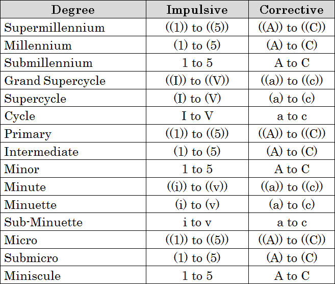
On the one hand, impulsive movements create trends and follow a sequence of five waves. On impulses, three waves move in the direction of the primary trend and two in the opposite direction.

On the other hand, a corrective movement consists of three waves; two of them will be in the opposite move to the main trend.

This eight-waves movement creates a cycle, and when it is complete, a new cycle of the same degree will start. In other words, when a five-waves and three-waves movement is complete, a new cycle of the same extension will take place.

Elliott gave intensive importance to corrections and told us the position of the market and the outlook. Elliott’s experience drove him to identify four main types of corrections as zigzag, flat, irregular, and triangles.

Making Simplifications

In the two latest articles, we discussed how we could simplify corrective patterns in the wave analysis using some chartist patterns as flags and triangles. Also, we commented on how it can help us in our study, reducing the time elapsed to develop a forecast and, finally, a trading plan.

The Analysis Process

The basic methodology to carry on the market analysis is to analyze from a higher to lesser time frame. In other words, we can start the study from a monthly range and finish in the hourly chart. Once we have identified the market structure, we begin to define scenarios that have a probability of occurrence. The scenarios are relevant to the analysis process because, using them, we can evaluate all possible price paths and decide which one of them is the most probable.

The Heating Oil Triangle

The following chart corresponds to Heating Oil in its weekly timeframe. In the figure, we observe the bullish sequence developed in three waves, which began on January 17, 2016, at $0.8552 per gallon. The energy commodity reached its highest level on October 03, 2018, at $2.4496 per gallon.

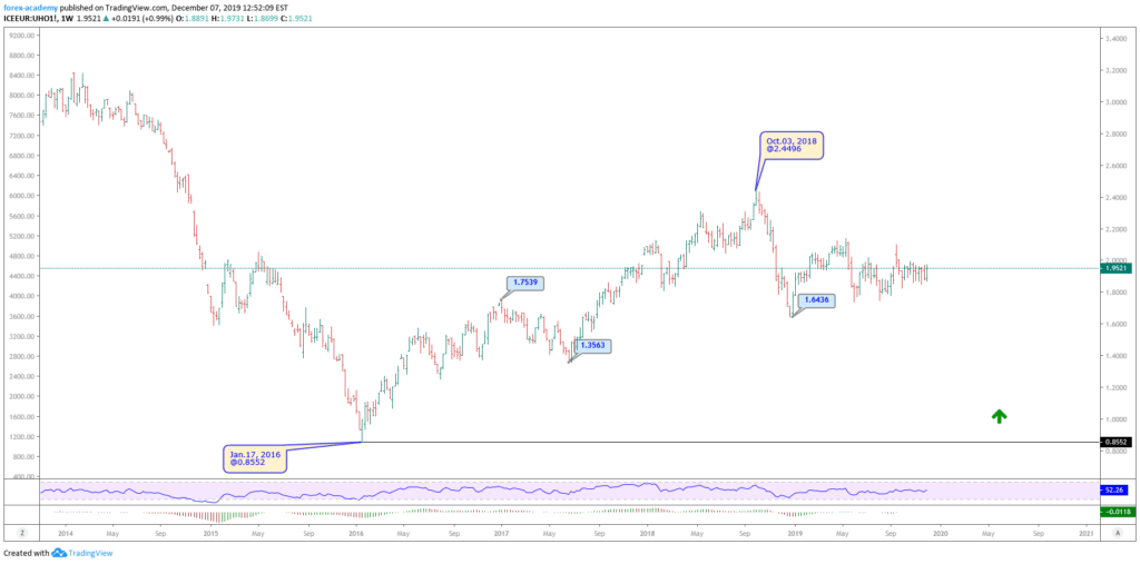
Once Heating Oil reached its high at $2.4496, the price started to make a bearish move, that found support at $1.6436 per gallon on January 02, 2019.

After that descent, the asset found buyers at $1.6436, Heating Oil’s traders started doing market swings. We can observe this as a triangle structure, as shown in the next daily chart.

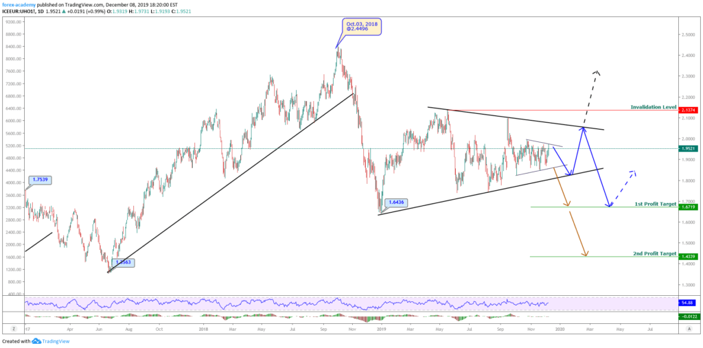
According to the Elliott Wave Theory, we know that a triangle structure has five internal segments which follow a 3-3-3-3-3 sequence. However, there is the possibility that the triangle pattern does not build a fifth inner leg.

Now, let us identify some scenarios for the next path on Heating Oil.

  • Scenario 1:The price moves down and crosses the base-line of the triangle (dark orange arrow), with a first potential profit target at $1.6719, and a second target at $1.4339 per gallon.
  • Scenario 2 (blue arrow) considers that Heating Oil drops and, then, bounces off from the base-line, but does not surpass the previous high at $2.0994. From there, the price action begins a new bearish wave that would drive the energy commodity to $1.6719 per gallon.
  • Scenario 3 (black arrow), considers that the price overcomes the resistance determined by the upper-line of the triangle and the invalidation level at $2.1374.

Conclusion

As we discussed in this article, the time dedicated to analyze and forecast a financial market is a valuable resource that could increase or reduce the hidden cost of the potential trade. As occurs in mathematical models, valid simplifications can help the analyst to reduce the time to a decision process.

Flags and triangles are simple and basic formations that can ease the market study.

Finally, the formulation of different scenarios provides a wide range of options about the next potential paths of the price action. Also, these scenarios create different answers facing the question of what if the market does that?
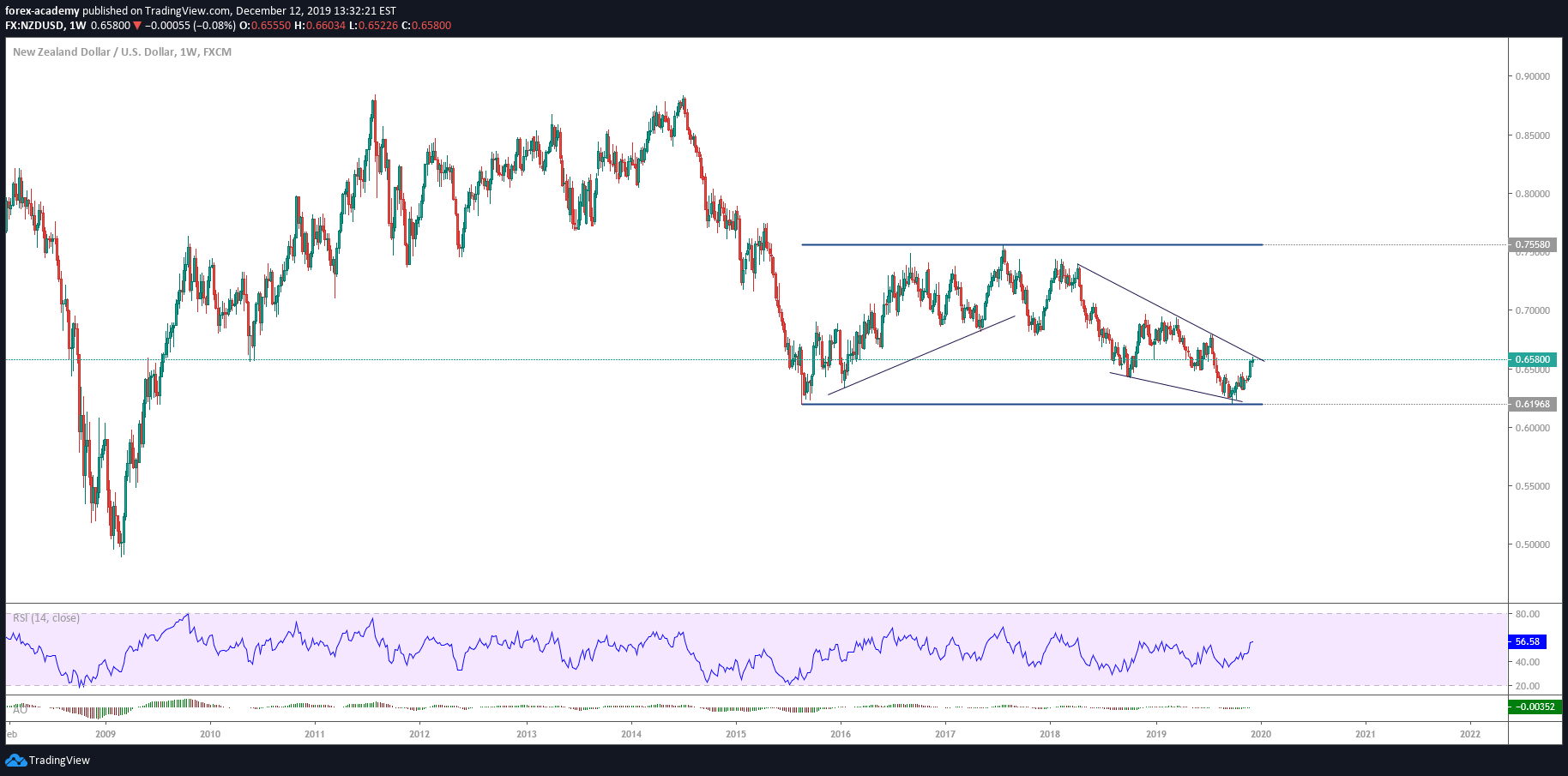
Categories
Forex Daily Topic Forex Elliott Wave

Analysis and Trading with Triangles

In our previous article, we discussed how we could simplify the zigzag and flat pattern by the chartist figure known as a flag. In this educational article, we will see how triangles can be used in wave analysis.

The Background

Within the Elliott wave theory, triangles represent one of the three basic corrective formations. Similarly, in traditional technical analysis, triangles represent consolidation and continuation formations of the trend.

Elliott defined triangles as a formation that have an internal structure subdivided into five waves following a 3-3-3-3-3 sequence. At its time, Elliott identified two triangle variations, which are classified as expansive or contractive.

In general terms, triangles represent the market indecision or the balance between the buying and selling forces.

The following chart shows the model of the triangles in their contractive and expansive variants, under the Elliott Waves theory and Traditional Technical Analysis perspective.

According to the point of view of the traditional technical analysis, we can observe that the triangle pattern is not forced to have five internal segments, as in Elliott’s wave theory. In consequence, a truncated zigzag or truncated flat structure could be simplified by a triangle pattern.

The Trading Setup

The trade configuration of a contracting triangle pattern has the following characteristics:

  • Entry Level: A buying (or selling) position will be activated if the price exceeds and closes above the swing of the previous top.
  • Profit Target: The first profit target level will take place at 78.6% of the Fibonacci expansion, while the second will be at 100%, and finally, the third profit target level will be at 127.2%.
  • Protective Stop: The invalidation level of the trade setup will be located below the lowest swing of the triangle pattern.

The trade configuration of an expansive triangle pattern has the following properties:

  • Entry Level: The trade will be activated if the price exceeds the height of the expanding triangle.
  • Profit Target: The first profit target level will be at 100% of the Fibonacci expansion. The second profit target level will be at 127.2%.
  • Protective Stop: The level of invalidation will be located below the lowest low of the expansive triangle pattern.

Examples

The following chart corresponds to the AUDUSD pair in its 12-hour timeframe. We can observe that the price action developed an expanding triangle formation, which began from mid-May 2019 and culminated in mid-July 2019.

From the chart, we detect that the expanding triangle reached its highest level at 0.70821, which corresponded to a false breakout. Subsequently, the price action resolved the next movement with a drop that took it to plunge until 0.66771.

The sell-side entry was activated once the price closed below the lowest level of the expanding triangle at 0.68317. Once activated the sales position, the price reached the first target at 0.67080.

Another possibility of entry that could be considered would be the closing below the last relevant swing, that is, the closing below 0.69105. This option could provide the trader with a higher profit compared to the risk taken compared to the original entry setup.

The next example corresponds to Silver in its daily chart. From the figure, we observe that the price made a record high early July 2016, reaching $21,225 per ounce, after this, the price action performed a corrective movement, once its found support, Silver built a tight contractive triangle.

After breaking below $18,715, Silver activated a bearish scenario that drove the price to fall to the third bearish target at $15.66 per ounce.

After having fulfilled the third bearish target, the price fell and reached $18.435 on April 17, 2017, where Silver began to build a contractive triangular structure that lasted until the end of June 2018.

Once the downward break of the long-lasting triangle occurred, we see that the price made a limited downward movement, which did not yield below $14 per ounce.

Conclusion

Based on the discussion of this article, we can conclude that regardless of the corrective structures that have three or five internal waves, these can be simplified as triangular patterns. Also, we can observe that a corrective wave or a short-range narrow triangle is likely to have an extended move that, in terms of Elliott’s wave theory, could correspond to an extended wave.

On the other hand, extensive triangular formations, or of a wide range, could lead the price to move in a range not as broad as in the previous case.

Finally, in the last example, we recognize how the alternation principle works in Elliott’s wave theory. Just as the first observed triangle is simple, and has a short duration, and the second corrective formation is extensive and complex.

Categories
Forex Elliott Wave

Corrective Waves and the Flag Pattern

Is it possible to simplify the wave analysis and compare it with classic chartist patterns? Identifying Elliott Wave patterns can seem confusing, especially if you are looking to differentiate between a flat or a zigzag pattern. In this educational article, we will look at some of Elliott’s patterns and compare them to traditional chartist figures.

The Normal Zigzag, Flat and the Flag Pattern

In the Elliott wave theory, the zigzag and the flat pattern are formations built by three internal waves. At the same time, depending on the strength of the corrective move, these could be more or less profound. The following figure shows the comparison between a normal corrective wave, which can be a zigzag or flat, and the flag pattern.

If we remember the wave theory, a zigzag pattern follows a 5-3-5 sequence, and the flat structure, a 3-3-5 internal subdivision. However, both formations can be simplified as a three-legs formation. Now, as we can see in the previous figure, the normal Zigzag and Flat structures can be simplified by a flag pattern.

The flag pattern is a chartist figure that represents a pause of the market trend and usually resolves as a continuation of the previous movement. The same situation occurs with the zigzag and flat pattern.

The flag pattern is spotted by a descending (or ascending) move, which connects in a tight range, its highs, and lows within a parallel channel.

The following chart exposes a series of flag formations detected on the GBPJPY cross in its 12-hour range.

On the figure, we observe that Flag patterns are commonly found in financial markets. According to Thomas Bulkowski’s publication, the flag pattern has a break-even or failure rate below 4%, which converts it as a “pretty nice” pattern to trade.

Flag Pattern Trade Setup

The flag trade setup is similar to the zigzag of flat configuration.

  • Entry: The trade is triggered once the price surpasses the end of wave “B,” or the previous swing high or low.
  • Protective Stop: The trade will be invalid if the price drops below the low of the flag.
  • Target: We will determine the profit target level using the Fibonacci expansion tool. The first target will be at the 100% level, as a second target at 127.2%, and the third profit target level will place at 161.8%

Putting All-together

The following chart illustrates the GBPCHF in its 8-hour range. In early January 2019, the cross developed a rally from 1.2248, which drove to the price until 1.2573. Once reached this high, the price action formed a corrective move in three waves. The bullish position was activated once price action surpassed the previous swing at 1.2524.

After the breakout, the price rallied over the three profit targets proposed. Note how the price runs when the flag pattern is tight and high, and the difference when the flag is broad in terms of price and time.

Conclusion

From the analysis realized, we conclude that a corrective structure as a normal zigzag or flat formation can be simplified as a flag pattern. This simplification could aid the traders in reducing the time analysis elapsed to the decision process before to place an order.

The confidence level of this pattern as a continuation figure could contribute to reducing the risk in the trading process.

Categories
Forex Elliott Wave

How to Use ETFs to Create Spreads

Exchange-Traded Funds, or better known as ETFs, are investment instruments that are traded in a centralized market. In this educational article, we will see how we can use them to create negotiating opportunities.

Exploring Markets and Diversification

In financial markets, there are virtually unlimited possibilities for investment. Decisions such as what to buy? What to sell? As well as the geographical region, level of risk, liquidity of the market or assets, expected profitability, among other aspects, are factors that an investor can face when planning his future investment.

Use of Intermarket Spreads

In simple words, a spread is a strategy on which the investor buys one market and sells another market simultaneously. For example, in the currency market, an investor could buy a contract of €100,000 and simultaneously sell a 100,000 euro on pounds sterling. In other words, this trade is equivalent to go long in the EUR/GBP spread.

Creating a Spread with ETFs

We can create different spreads according to the market in which we are interested in investing. To this end, the decision criteria will be those ETFs with higher liquidity. The following tables represent ETFs that are associated with commodities, particularly Gold and Silver.

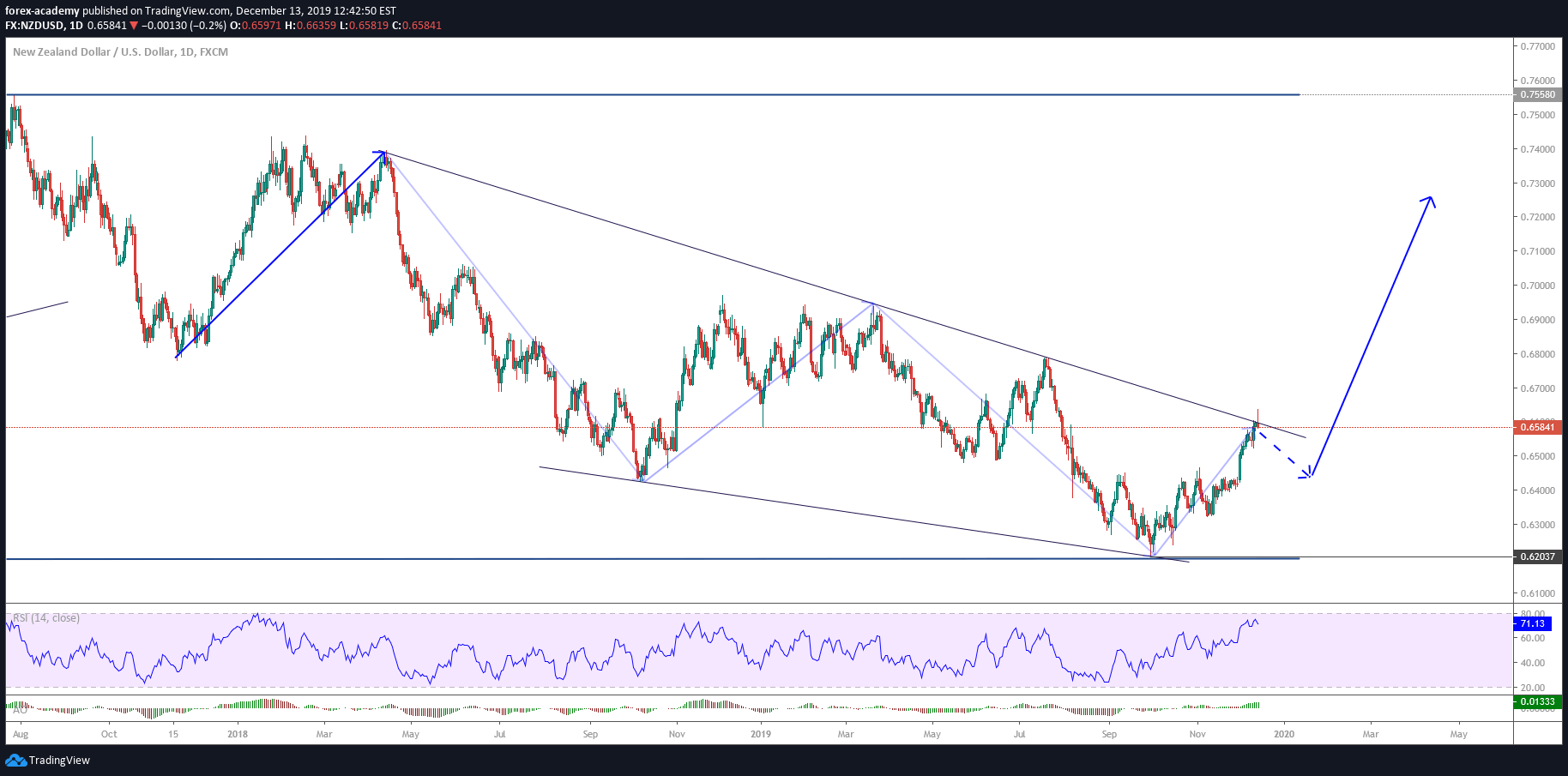
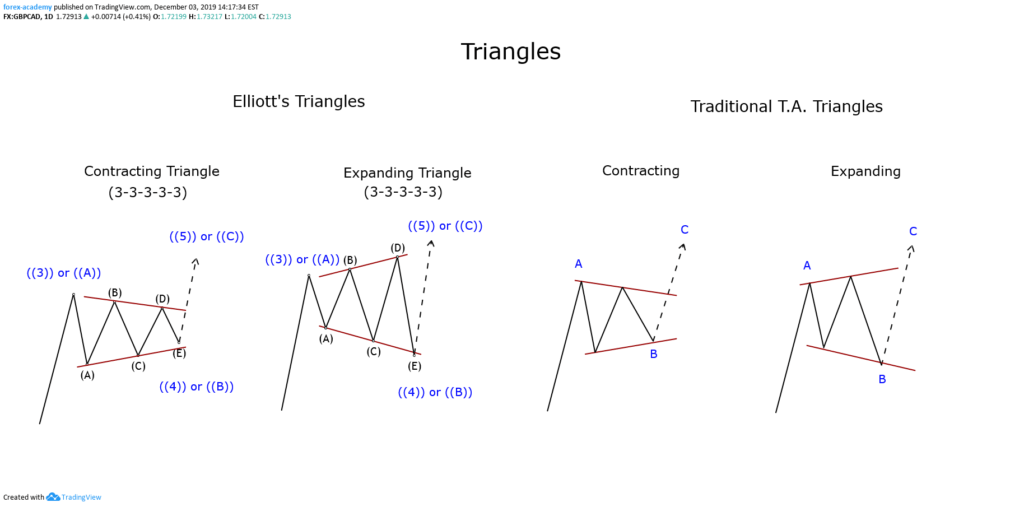
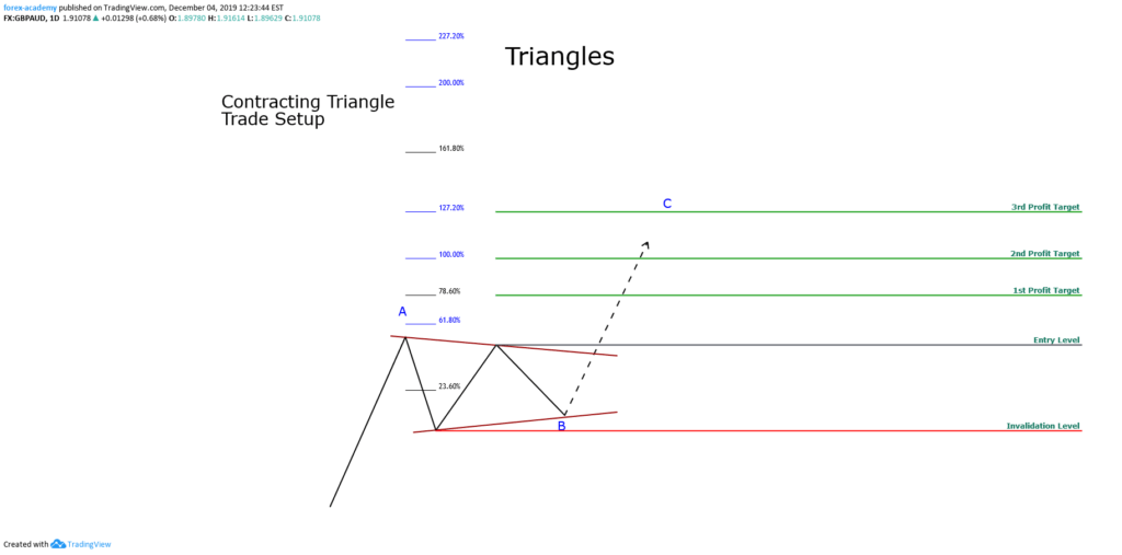
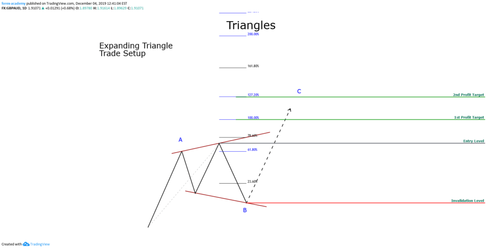
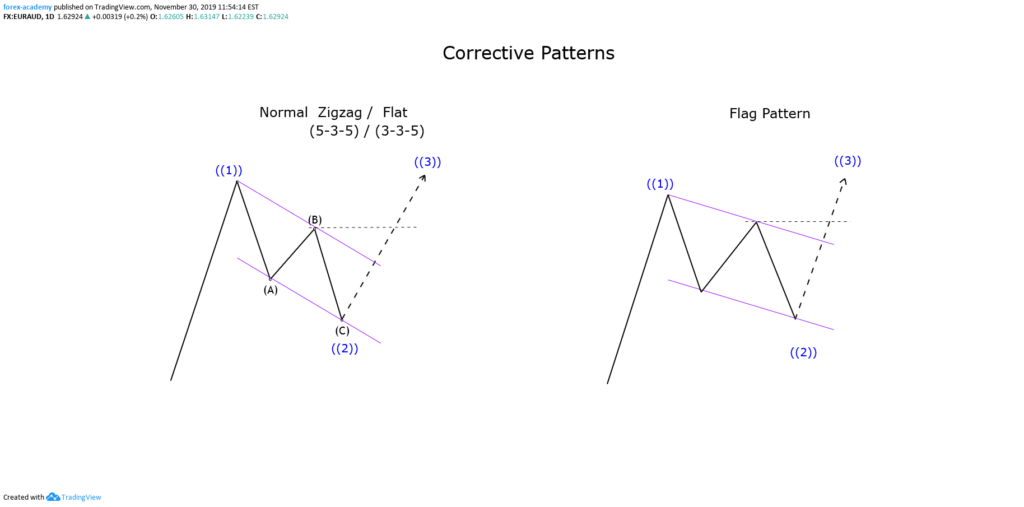
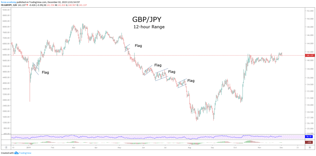
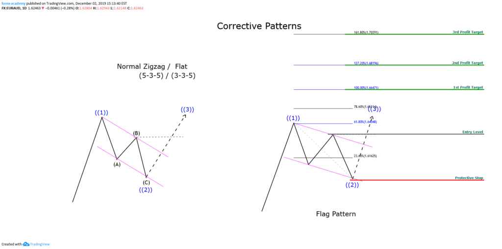
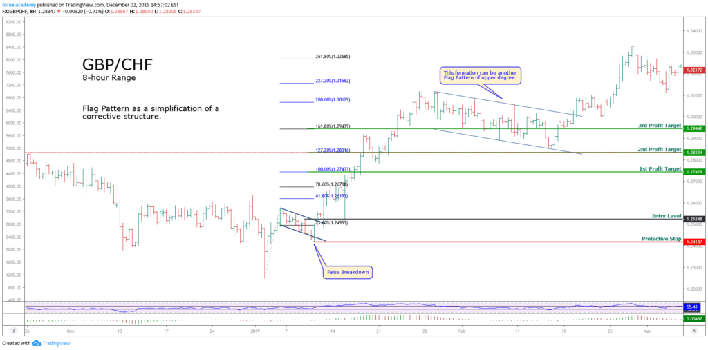
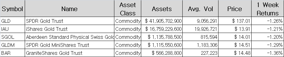
Table 1 – ETFs Based on Gold

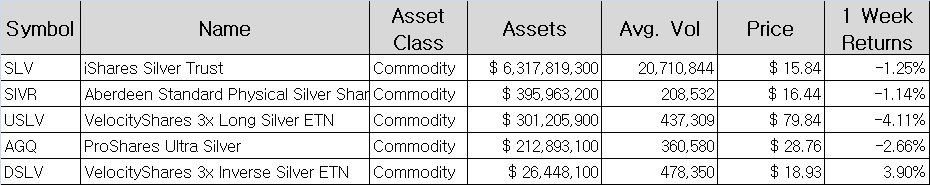
Table 2 – ETFs Based on Silver

From tables 1 and 2, we see that ETFs GLD and SLV record the largest size in each group. Consequently, they will be used for the construction of the GLD/SLV spread.

The GLD/SLV spread in its daily chart shows both precious metals developing a corrective structure as a B wave. Therefore, the Gold/Silver spread could see a new low. In other words, we expect a decline in GLD and an upside in SLV.

The following example shows the spread between SPY and QQQ in its daily chart. The ETF SPY is characterized by replicating the S&P 500 index, while QQQ replicates the NASDAQ 100 index.

In the spread graph SPY/QQQ, we detect that the price is developing an Ending Diagonal structure in a bearish cycle. Also, although QQQ continues to push downwards in front of the SPY, it should be noted that this pattern is an exhaustion formation. Thus, it is likely that these markets reverse soon. In this case, the positioning strategy would be a long position in SPY and another short position in QQQ.

Conclusion

After the analysis made here, you may see that everything traded, including pairs, can be considered as spread bets between an asset the underlying payment method. It is just that, considering the relative stability of fiat money it makes more sense to use the term spread when exchanging two volatile assets, as one of the main objectives of spread bets is to tame the overall market volatility since the investor is selling and buying volatility at the same time.

According to what here is exposed, the creation of spreads can help explore the strength/ weakness situation between markets. Likewise, the exercise could help to make decisions on which assets to choose. It should be emphasized that before entering a market, the  spread’s price action must confirm the movement that is predicted.

Finally, this type of analysis can be extended to the futures market between futures contracts with different or similar expirations. This kind of analysis can also be applied in the stocks market, bonds, etc.

Categories
Forex Elliott Wave

The USDJPY and its 3-Year Triangle

The triangle is one of the three basic corrective patterns along with the Flat structure, with more variations within Elliott’s Wave Theory. In this educational article, we will review the basic concepts of the triangle pattern and then apply it to the USDJPY pair.

The Fundamentals

Triangles are one of the three basic corrective formations described by R.N. Elliott. Five internal segments characterize them. The inner legs overlap and follow an internal sequence as 3-3-3-3-3.

The following figure shows the different types of triangles. By simplification, we omitted the internal structure of each segment that composes the triangle pattern.

We should consider the nature of the triangle, a balance between the buying and selling forces. In this context, and under a conservative approach to trading, it is not desirable to trade within this internal structure. However, the breakout of price action across the wave (D) can provide a reliable entry to the market with reduced risk.

The 3-Year Triangle of USDJPY

The following chart corresponds to the USDJPY pair in its weekly timeframe, using a log scale. We observe the price action on the Japanese currency developing a Contracting Triangle structure that began at the end of 2016.

The next chart shows the USDJPY moving in a 12-hour timeframe. The pair shows the last internal segment corresponding to a wave (E) of Intermediate degree labeled in black.

At the same time, in the last figure, we can distinguish the price action developing an Expanding Triangle formation in a wave C of Minor degree labeled in blue. However, the RSI oscillator reveals in its progress the shape of a contractive triangle pattern.

It should be noted that when the price action develops an Expansive Triangle in a wave C, the pattern should correspond to an Expansive Diagonal formation. Remember that a diagonal pattern has five internal waves overlapped one with another. At the same time, each inner leg holds three segments.

Trading the USDJPY Triangle

The USDJPY pair in its 12-hour chart shows an incomplete expansive diagonal. Consequently, positioning on the long-side could still have endeavored with a short-term objective placed in the upper trendline of the diagonal. A likely target area would be between 109,716 and 110,551.

Considering that the invalidation level of the bullish segment is the bottom of the wave ((iv)) in green at 108,242, the breakdown and close of the price below this level could give us the first bearish scenario with a target at the end of the wave B labeled in blue located at 106,625.

Now, if the USDJPY price continues extending its falls below the end of wave C in blue and (D) in black located at 104,446, a major-degree bearish scenario would be activated. Under this context, the pair could see the psychological support of 100 yen per dollar.

Conclusions

Depending on the trader’s style and its risk aversion, the internal structure of the triangle pattern could be traded one timeframe shorter than the time frame in which the triangle has been identified.

We must remember that the internal structure of the triangle follows a sequence 3-3-3-3-3. Under this context, a three-wave corrective structure can be a Flat pattern (which has a subdivision 3-3-5); or it can also be a zigzag pattern (5-3-5). Therefore, an internal wave C could give a trading opportunity. However, knowing the nature of the triangle pattern, and considering it is formed by the struggle between buyers and sellers, the targets of the movements anticipated should be limited by the triangle formation.

Categories
Forex Elliott Wave

Dollar Index and the Alternation Principle

In our article “Impulsive Waves Construction – Part 1,” we introduced the concept of “alternation.” In this educational article, we’ll apply this concept to the Dollar Index Analysis.

The Alternation Principle

Just as the Wave Principle obeys a law, alternation is also the law of nature. We can observe this law both in the universe as human activities. Just as the seasons of the year or the phases of the Moon alternate, socio-economic activities also alternate.

There is probably no other activity that has devoted as many resources to its study as financial markets. An example where we can observe the principle of alternation is in the U.S. Dollar Index.

Application in the Dollar Index

The U.S. Dollar Index (DXY), in its daily chart, illustrates the bullish sequence he developed since it found buyers on February 16, 2018, and drove to the price from 88.25 until 99.67 on October 01, 2019.

From the chart, we can observe how DXY performed the rally in two stages. In each phase, we see how the advance alternates in both price and time. In particular, the first rally was run in 180 days and advanced by about 9.9%. The second tranche lasted 376 days and increased by 6.22 percent.

Our reader can observe the same situation in the daily chart of the EURGBP cross, which was discussed in the educational article “How to analyze a fast market using the Elliott Wave Principle.”

Looking at the second chart, our reader can appreciate how price and time alternate their relationship in the EURGBP cross.

Alternation and the Analysis Process

An approach to simplify the analysis process consists of identifying different parts of the movement developed by the market and analyze it part by part. The next DXY daily chart illustrates this process.

The following 4-hour chart exposes the advance developed by the Dollar Index once it found buyers at level 88.25.

From the chart, we observe a first impulsive upward movement labeled ((i)) in black, which developed five waves of a lesser degree. Once DXY completed the first wave, the price corrected by a wave ((ii)), which is divided into three internal segments labeled as (a), (b), and (c) in blue.

Within the corrective structure, alternation over time can be distinguished. For example, the wave (a) in blue ended in 23 bars, the wave (b), in turn, was developed in 57 bars. Finally, the wave (c) took 26 bars to finish. This time difference reflects the principle of alternation in terms of simplicity and complexity of each segment that composes the price movement.

The following chart shows how the action of the price alternates in the waves (ii) and (iv) in blue. In the wave (ii), the corrective movement of DXY developed in 43 bars, while the wave (iv) was completed in only 19 bars.

Conclusions

Based on the case studied, we can recognize how the principle of alternation is reflected in the financial markets and different temporalities. This application in different time frames allows us to identify the concept of “market fractality.”

On the other hand, we can observe how the market alternates not only in a price dimension but also in time. In other words, the progress of the market must be studied concerning both price and time.

Finally, if the range of a movement is narrow and has a relatively long duration, the next move will likely be broad in terms of price motion and shorter in length.

Categories
Forex Elliott Wave

How to Analyze a Fast Market Using the Elliott Wave Principle – Part 2

In our previous article, we introduced the concept of “fast market.” Also, we commented about the importance of watching the big-picture to support the market’s general overview. In this educational article, we’ll review the analysis of the fast movement.

Disclosing the Speed

Once the market moved following our forecast, the price action developed its next sequence in a fast way. To aid in building our analysis in the EURGBP cross, we’ll use the RSI indicator to identify each swing.

From the EURGBP hourly chart, we observe the bullish sequence started on May 05. The RSI use, allows us to identify each swing of waves 2 and 4, and divergences the end of waves 3 and 5.

Until now, the movement developed by EURGBP corresponds to a 5-3 sequence; thus, the next path should develop in five waves. In consequence, our new hypothesis could be the next move a wave three or be the second leg of a zigzag pattern.

The second EURGBP chart exposes the progress in an ending diagonal pattern. This Elliott wave formation is a motive wave built by five internal legs that overlap each other.

On the other hand, the new big-picture structure observed on the EURGBP cross unveils a 5-3-5 sequence. Thus, according to the Elliott wave principle, this formation corresponds to a zigzag pattern.

Another observation comes from the alternation between the first and second bullish leg. Both segments moved on a different relationship price and time. In other words, while the first leg ascends in a fast step, the second one progress at a slower price/time relation.

Now, from the Elliott wave principle, the next path from the EURGBP should be a corrective move in three waves. If the price breaks below the invalidation level, the correction should be more profound.

On the following chart, we observe an incomplete corrective move developed in two internal waves labeled in black. In consequence, the next movement should be a wave ((c)) in black. The completion should complete a new wave A labeled in green.

Until this moment, the price action bounced above the invalidation level, which makes us observe two things:

  1. The EURGBP cross is running in a complex corrective structure, likely a double three pattern. This Elliott wave structure is labeled as WXY, follows a 3-3-3 sequence, and develops seven swings.
  2. Probably according to the alternation principle, the next corrective structure could be a flat pattern.

The following chart exposes the waves A and B labeled in green completion. As can be noted, wave A holds three internal legs, wave B retraces between 81% and 100% of A. Thus, the Elliott wave structure should correspond to a regular flat pattern.

Finally, the next EURGBP chart illustrates the end of the last segment of the wave C from the regular flat pattern, which is part of a complex corrective sequence, in this case, the formation corresponds to a double three structure.

As a learned lesson, the use of the RSI indicator is useful to support the wave identification process. Similarly, to apply the Elliott Wave Principle is essential to know the basic corrective patterns to follow any market. Finally, remember that the market has only two ways to move: it moves in three or five waves.

Categories
Forex Elliott Wave

How to Analyze a Fast Market Using the Elliott Wave Principle – Part 1

The speed is a characteristic of nature; in the same way, some markets tend to be faster than others. The problem arises when a market moves sharply. In this educational article, we’ll introduce how to analyze a fast market using the Elliott Wave Principle.

Price and Speed

Both price and speed are individual characteristics of each market. Depending on specific factors, one market could be faster than another.

The problem arises when, in an active market, the price moves faster than usual. R.N. Elliott, in his Treatise “The Wave Principle,” wrote:

“In fast markets, it is essential to observe the daily as well as the weekly ranges; otherwise, characteristics of importance may be hidden.”

In other words, when the market studied in a specific timeframe doesn’t allow to identify any pattern. It is useful in these cases to observe the market in a higher time frame, for example, the daily or weekly timeframes.

The Case of Study

Consider the EURGBP cross in its 4-hour chart, which shows a rally developed from early May until the middle of August 2019. The remarkable observation is that the first part of the rally was faster than the second part of the range of study.

As a first step, let us observe the big-picture; in this case, we will study the EURGBP cross in a weekly timeframe. As can be noted, the EURGBP developed an extended Wave 3.

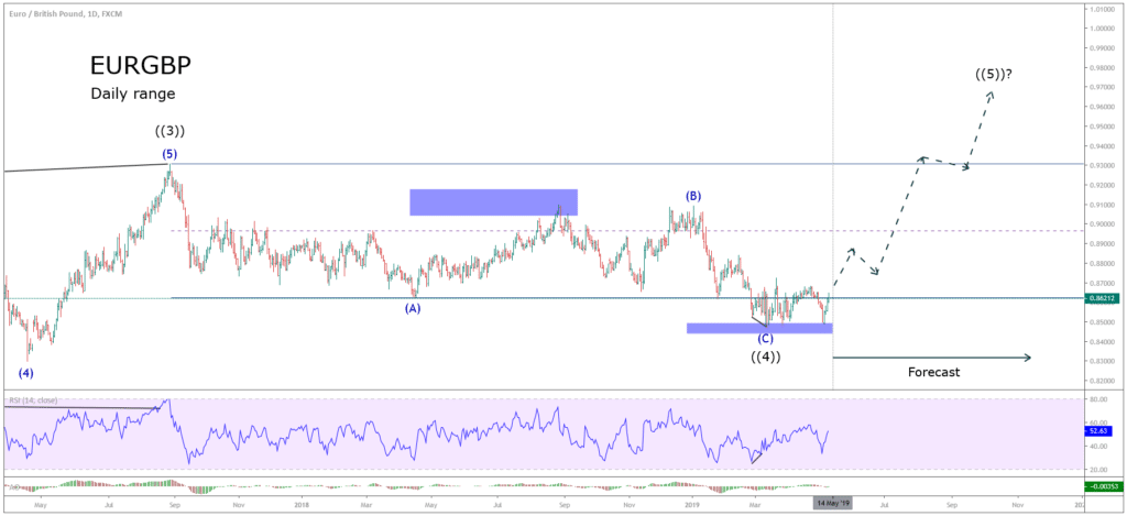
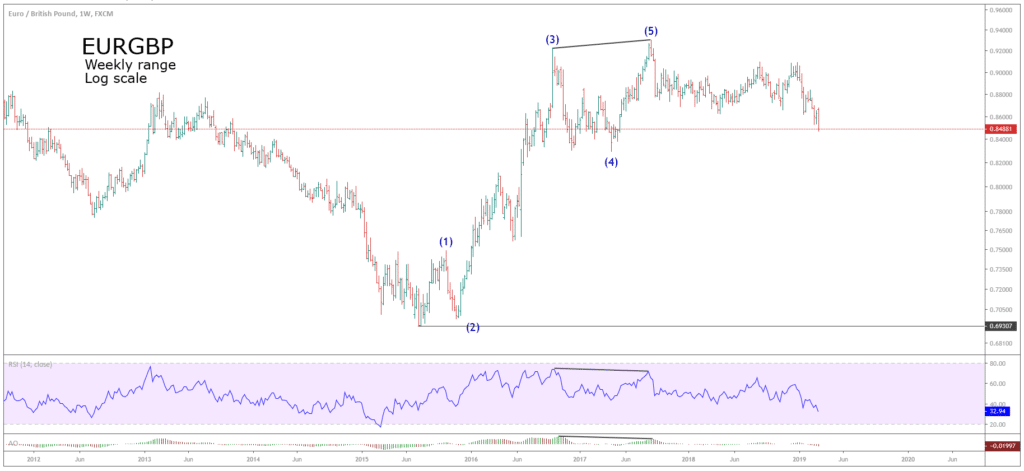
Both the RSI and the Awesome Oscillator display a bearish divergence, that helped us to identify waves (3) and (5).

In consequence, in view that the five-wave sequence has been completed, it is time for a corrective movement in three waves.

The next chart shows the possible recount of the EURGBP cross.


In the above figure, we observe that the cross could have fully completed a cycle that, as we know, includes a motive impulse and its corrective sequence. Thus, if our market hypothesis is that the EURGBP has completed a cycle, then our forecast should consider a new five-wave rally.

The following chart unveils the upward movement developed by the EURGBP from its bottom, established in early May.


In the next educational article, we will expand the analysis on how to decipher a fast market using the Elliott Wave Principle.

Categories
Forex Elliott Wave

Understanding the Flat Pattern

The flat pattern is a corrective formation that runs in a 3-3-5 sequence. Also, compared with other Elliott wave patterns, it has the most extensive variations. In this educational article, we will review the characteristics of the flat correction and its varieties.

The Broad Concept

The flat structure is one of the three basic corrective patterns described by R.N. Elliott in his hork “The Wave Principle.” This formation has an internal 3-3-5 sequence. The next figure illustrates the basic concept.

The main characteristic of the flat pattern is that wave B tends to extend more than 61.8% of wave A.

Even wave B can surpass 100% of wave A. Depending on its extension, wave B will be weak, regular, or strong. As a summary,

  • Wave B is Weak if wave B retraces between 61.8% and 81% of wave A.
  • Wave B is Regular if wave B retraces between 81% and 100% of wave A.
  • Wave B is Strong if wave B retraces more than 100% of wave A.

On the other hand, wave C must be above or equal to 38.2% of wave A. Additionally, wave C tends to variate its extension depending on the wave B strength.


  1. Strong Flat: If wave B retraces over 100% and less than 127.2% of wave A, likely, wave C completely retraces wave B.
    In case that wave B retraces more than 127.2% of wave A, it is highly probable that wave C does not retraces completely wave B.
  2. Regular flat: It occurs when wave B retraces between 81% and 100%. In this case, it is highly likely that wave C retrace completely wave B.
  3. Weak flat: In case that wave B retraces between 61.8% and 81% of A, it is possible that wave C retrace over 100% of wave B.

Measuring the Flat Pattern

The Gasoline daily chart illustrates a flat structure. The measuring process of wave A makes us observe that wave B retraces between 618% and 81% of wave A.

In consequence, as said previously, the corrective pattern corresponds to a weak flat structure. Thus, we should expect a wave C that retraces over 100% of wave B, as shown in the following chart.


In summary, the measuring process of wave B of a flat pattern is a useful process that could allow you to identify the potential extension of wave C.

Categories
Forex Elliott Wave

Elliott Wave Principle – Advanced Concepts – Part 3

The Relative Strength Index (RSI) indicator was developed in 1978 by J. Welles Wilder. the RSI is a Momentum indicator that measures the change of the price movement. In this educational article, we will review how to apply the RSI with the Elliott Wave Analysis.

The basics

Possibly, the RSI indicator is the most widespread indicator from professionals to retail traders. The RSI is an oscillator that moves in a range between 0 to 100. Alexander Elder describes it as a “leading or coincident indicator – never laggard.”
 
Some applications of RSI are tops and bottoms identification, divergences, failure swings, support and resistance, and chart formations.
 
In the Elliott wave theory, the RSI application can to aid in the wave identification process. In particular, the identification of divergences is the most used application in the wave analysis.
 
J. W. Wilder describes the divergence between the price action and RSI path as a “powerful indication that the market could reverse soon.
 
A divergence takes place when the price is still increasing, while the RSI began decreasing (bearish divergence). Or when the price falls, and the RSI climbs (bullish divergence.) In the wave analysis terms, divergences appear between the end of waves three and five. Let’s see a couple of examples.

RSI and the Elliott Wave Principle

Johnson & Johnson (NYSE:JNJ), on its weekly chart, illustrates the RSI and the Awesome Oscillator. Both indicators show the divergence created between the end of waves three and five.

On the JNJ chart, we also can observe the RSI levels when price action runs in a wave three. When this occurs, the RSI tends to move between the levels 70 and 80.

In a bull market scenario, usually, the price action tends to find support near to level 40. When the price moves in a bear market, the ascending correction tends to find resistance near to level 60. This concept, with the swings identification, can support the wave analysis.

The following chart corresponds to the Dollar Index (DXY) in its 8-hour timeframe. From the figure, we observe the bullish sequence developed in five internal legs, in which we observe that each leg has three waves.

As a conclusion from the study using the RSI indicator and wave analysis, the price action unveils an ending diagonal pattern. The Elliott wave structure shows us that the Greenback should see new lower lows.

Categories
Forex Elliott Wave

Elliott Wave Principle – Advanced Concepts – Part 2

Indicators are a useful tool that can aid in supporting the analysis process. In this educational article, we will review the Awesome Oscillator and how it can help us in an Elliott Wave study.

The basics

The Awesome Oscillator (AO) is also known as the Elliott Wave oscillator, was developed by Bill Williams. The AO measures the immediate momentum of the five previous periods, compared with the momentum of the last 34 periods.

The calculation is based on the simple moving average of the midpoint (HL / 2) of 34 periods minus the simple moving average of the midpoint of 5 periods.

Elliott Wave and the Awesome Oscillator

The following chart corresponds to the Johnson and Johnson (NYSE:JNJ) weekly chart. The bullish motive wave started with the August 2015 low at $128.51 per share. From this low, JNJ began to a bullish sequence, which drove it to reach the $148.32 level.


From the AO oscillator, we can recognize the following elements of the price action:

  1. Trend bias: If the trend is bullish, the AO will be positive. If it is bearish, the oscillator will move on the negative side. For our example, the market direction of the range of time studied corresponds to a bullish trend.
  2. Wave three: We can identify wave three with the most prominent distance of the AO. From the JNJ example, we distinguish a wave (3) of Intermediate degree labeled in black. At this point, the stock reached $125.90 per share. After this peak, JNJ started a corrective sequence, and the oscillator began to decrease, even moved in the negative side.
  3. Wave five: In the same way as the third wave, we can recognize the fifth wave watching the AO because momentum follows the dominant trend. However, in this segment, the oscillator shows a divergence between the peaks of waves three and five. In our example, JNJ ended the wave (5) on the half of January 2018 at $148.32 per share. We can observe the bearish divergence between the price and the oscillator.
  4. Corrective waves: We can use the AO to identify corrective waves watching how it decreases against the prevailing trend. From the JNJ chart, the oscillator turns negative when the price develops a retracement.

In summary, the Awesome Oscillator can be a useful tool to complement the EW analysis, especially in wave identification. A divergence involves the exhaustion of the movement, but the price is not compelled to reverse the trend.

Categories
Forex Elliott Wave

Elliott Wave Principle – Advanced Concepts – Part 1

Intermarket Analysis studies the correlation or relationship between different markets or assets. In this educational article, we will review how to apply the correlation analysis within the Elliott Wave Principle.

The basics

In financial markets, we use the correlation to measure the relationship between two or more assets. These assets can be from the same or different markets.

For example, we can analyze the relationship between a commodity and a currency pair. In the first figure, we observe the relationship between Crude Oil (NYMEX:CL) and the FX pair US Dollar – Canadian Dollar (USDCAD).

From the figure, we observe that Crude Oil holds an inverse relationship with USDCAD. It means that, if CL soars, the USDCAD should decrease, and vice-versa. This type of correlation is known as negative or inverse correlation.

In the contrarian case, when an asset moves in the same direction that the second one is known as positive or direct correlation.

The second key concept in the Intermarket analysis is convergence and divergence. In the same way that we use and identify divergences, or deviations, on technical indicators, we use it with correlations. Divergences allow us to foresee the exhaustion of a sequence.

From the figure one, we identified the divergence with the red arrow. In the example, we observe at the end of a wave, when Crude Oil soars, the Loonie decreases. In general, we find divergences when the fifth wave is in progress.

Putting all together

The next chart corresponds to the NASDAQ Biotechnology ETF (IBB) and the stock price chart of MERCK & Co. (MRK), in the weekly timeframe and log scale.

In this case, both assets belong to the same sector. Thus, we expect a positive correlation with each other. From the chart, we observe that IBB and MRK started a rally in the third quarter of 2009.

MRK looks like it’s near to end the bull trend; however, IBB unveils an incomplete bullish five-waves sequence.

Finally, please, note how the divergence appears at the end of the third wave on IBB, while MRK started the wave four.

Categories
Elliott Wave Guide Forex Elliott Wave

Essential Elliott Wave Theory Guideline

Recently, we ended the series that presents the basic concepts of the Elliott Wave Theory. In this guideline, we disclose the contents developed.

  1. Fundamentals of Elliott Wave Theory. Divided into three parts, we introduce the basic concepts of the wave principle.
    1. Wave principle and the five-waves structure.
    2. Motive waves, corrective waves, and cycles.
    3. Degrees and labeling.
  2. Planning the First Wave Analysis. In this two-parts chapter, we explain the necessary steps to analyze using the Elliott wave principle.
    1. Setting charts and the identification process.
    2. Proportionality and the relationship between price and time.
  3. Impulsive Waves Construction. This section offers the key concepts to understand the nature of impulsive waves.
    1. Nature of impulsive waves and the alternation principle.
    2. The channeling process.
    3. Extensions.
    4. Leading and Ending Diagonal.
  4. Corrective Waves Construction. Elliott, in his Treatise, spent a large part of time describing corrective waves. In this section, we present different corrective formations.
    1. Nature of corrective waves and alternation.
    2. Zig-zag pattern.
    3. Flat pattern.
    4. Triangles.
    5. Complex corrective waves.
  5. Elliott Wave Theory and Fibonacci. In this one-part article unfolds the keys to use Fibonacci retracement and expansion tools.
  6. Trading the Elliott Wave Principle. We end the cycle of the Elliott wave theory with the five-part guidelines.
    1. Wave three structure trading setup.
    2. Wave five and ending diagonal trading setup.
    3. Zig-zag pattern trading setup.
    4. Flat pattern trading setup.
    5. Triangle formation trading setup.
Categories
Forex Elliott Wave

Traders’ Guide to the Elliott Wave Theory

The Elliott wave principle has its origin in the early 1930’s decade. The introduction of the wave concept was published in 1934 by R.N. Elliott in his work “The Wave Principle.”

The Wave Principle

In Elliott’s treatise, the author indicates that financial markets as a socio-economic activity hold a specific structure composed of five waves. In his model, Elliott teaches us that waves 1, 3, and 5, move following the direction of the dominant trend. On the contrary, waves 2 and 4 develop an opposite movement to the primary trend.

Parts of the Cycle

The Elliott wave cycle has two components; these components are an impulsive wave and a corrective wave.

As said before, an impulsive sequence holds five waves; and a corrective wave contains three segments. In consequence, a complete cycle has eight waves.

The next figure unveils a complete Elliott wave cycle.

The Analysis Process

When R.N. Elliott developed its theory, he defined a specific terminology to maintain the order in the analysis process. The author established a series of degrees that must be considered in relative terms about price and time.

The next table illustrates the different degrees defined by Elliott.

The analysis process starts with the relevant highs and lows identification in a larger timeframe. After this, we proceed to study the prices’ sequence; to aid to do this step, we examine the proportionality and the relation between price and time. The next chart illustrates the relationship between price and time.


The next stage is to identify impulsive waves. The basic guidelines of motive waves are:

  1. It has five consecutive segments building a trend.
  2. Three segments move in the same direction.
  3. Wave three never is the shortest.
  4. Wave two never ends below the origin of wave one.
  5. When an impulsive movement finishes, it starts a corrective move of the same degree.

Alternation is a key concept of the wave principle. We observe the motive and corrective waves alternate one with another.

We observe the alternation in:

  • Distance.
  • Time.
  • Retracement.
  • Complexity.

The following EURAUD charts illustrate the concept of an alternation.

Categories
Forex Elliott Wave

Trading the Elliott Wave Principle – Part 5

Triangles are the third fundamental Elliott wave corrective structure. In this educational article, we will review the guidelines to trade this pattern.

The basics

The triangle structure is a corrective formation with a 3-3-3-3-3 internal sequence. Triangles usually tend to appear in waves four and B.

In this formation, volume tends to decrease as the triangle progresses. Also, it characterizes by the balance between bull and bear traders.

The following figure illustrates the trading setup for a contracting triangle. The entry is triggered once the price action strikes and closes above the end of wave (D) labeled in black degree.


To place the potential targets, we can measure the Fibonacci projection from the origin of wave ((3)) or ((A)) labeled in red, and the lowest level of the triangle. The first target will be at 61.8%, and the second target at 100%.

The trading setup is invalid if the price pierces the wave (A) labeled in black degree.

Golden triangle

Gold, in its weekly chart, shows the guideline of an Elliott wave contracting triangle in progress. The bullish sequence starts on November 30, 2015, once the yellow metal found buyers at $1,046.54 per ounce.

The golden metal made the first rally until early July 2016 at $1,375.15 per ounce. After this move, Gold made an up and down sideways movement till late April 2019.

Now that we have identified the start of a price cycle, we have to face the question, “do I recognize an Elliott wave pattern?”

In this case, we start from the most straightforward formation, which could correspond to a Contracting Triangle.


Now that we have recognized a wave pattern, we advance to the second stage, which is to define our trading plan. Following the triangle setup guideline, we have to expect the breakout of wave (D) labeled in black at $1,346.75.

The theory says that the first profit target must be at 61.8% of the Fibonacci projection. However, this level is under the entry-level. In this case, we place the first profit target at the 100% level at $1,453.78. The second profit target will be at the 127.2% level at $1,543.80 per ounce.

The invalidation level is theoretically below the wave (A) labeled in the black degree at $1,122.10.

Now that we have defined the trading plan, the third stage is to manage the trade and risk. The first step is to reduce the risk. In this case, we move the protective stop from the theoretical invalidation level to the end of the wave (E) at $1,266.39, as shown in the next figure.


Once that we have reduced the risk and the trade advances, the trader must eradicate the risk. In this example, after Gold reached the first profit target at $1,453.78, we move the protective stop to the entry-level.

As an alternative to eliminate the risk, the protective stop could be placed considering the entry-level plus the trade costs, for example, commission costs and swap.


The last step of the trade management, before the trade reaches the final profit target, is to protect open profits. This last stage depends on the criteria of each trader.

Categories
Forex Elliott Wave

Trading the Elliott Wave Principle – Part 4

The flat pattern is the second fundamental Elliott Wave corrective structure. In this educational article, we will review the guideline to trade the flat structure.

The basics

Flat pattern is an Elliott wave corrective structure built by three waves, and its internal sequence is 3-3-5. There exist a single model to trade a flat formation. The following chart shows the trading setup of a flat corrective structure.


From the basic model, the entry is given once price action breaks and closes above wave 4 labeled in blue, of wave (C) labeled in black. The profit target is placed in the same way as the zig-zag trade setup. It is at 100%, 127.2%, and 161.8% of the Fibonacci projection of waves ((1)) and ((2)) labeled in red. The invalidation level is under the end of the wave (C).

Trading the flat pattern

Before to define place an order, we must answer the question, “Do I see some Elliott wave pattern?”.

In the example, the IBM (NYSE:IBM) in its 8-hour chart shows a first five waves bearish sequence started on April 10, 2014. Once IBM founded buyers on January 29, 2015, at $149.52 per share, the price developed a three waves movement as a flat pattern, which ended at $176,25 on May 04, 2015.


If our hypothesis is correct, it is the Elliott wave pattern recognized is a flat structure, we can do our trading plan. The entry should be placed after the completion of the second wave (B) or (2) labeled in black degree.

The short position is triggered after the breakdown and close below the last swing at $168.75. The target is defined using the Fibonacci projection between (A) and (B) waves. In our example, IBM reached the first target at $126.53 on 100% of the Fibonacci projection.

The third part of the trade is to manage the risk of the trading plan. The first stage is to reduce the risk; for this stage, we set the invalidation level above the end of wave (B) or (2) at $176.25. Once IBM plummets, we eliminate the risk after the price drops into the 61.8% of Fibonacci projection at $145.60.

Finally, we have to protect the open profits, for example, each $5 of advance, we can move the protective stop each $5 of progress.

Categories
Forex Elliott Wave

Trading the Elliott Wave Principle – Part 3

The zig-zag pattern is a corrective Elliott Wave structure developed by a 5-3-5 internal sequence. In this educational article, we will unfold two guidelines to trade this pattern.

Looking at the wave B

The first guideline is looking at wave B with the eyes placed in wave C progress. The following chart shows an idealization of this trading setup.


There are two different ways to set up the entry into the market. The first one is to wait for the retrace of wave (B) into the area between 38.2% and 61.5% of Fibonacci retracement. The second one settles once the price breaks and closes below wave B of wave (B). In the chart, wave B has a blue label, and wave (B) has a black degree.

The invalidation level is above wave 5, or the last swing. To set the profit target, we use the Fibonacci projection. The first target (conservative scenario) is at the 61.8% of waves (A) and (B). The second target is at 100%, and the last one is at 127.2%.

Following the trend

The second guideline is at the end of wave C. In this context; we seek to join the primary trend. The next chart explains the model for this setup.


The setup is as commented in the article “Trading the Elliott Wave Principle – Part 1.” In this case, from the previous chart, we enter the market after the breakout and close of wave 4 of wave (C).

The first profit target is at 100% of the Fibonacci projection of waves ((1)) and ((2)) labeled in red degree. Note that a conservative profit target could be at the 61.8% of the Fibonacci projection.

An alternative to placing the invalidation level is below the end of wave (C). A second option is under the origin of wave ((1)) labeled in red degree.

Trading the zig-zag pattern

The Bank of America Corp. (NYSE:BAC) 3-hour chart shows a zig-zag structure. The Elliott Wave formation started on December 31, 2014, when the price found sellers at $18.21 per share.


Sometimes, the line-chart can be helpful to unveil the internal structure. From the BAC line chart (left), we observe the 5-3-5 sequence started at the end of December 2014.

On the right side, we see the OHLC chart. In this figure, we observe the trading setup looking for trade the wave C.

From the example; the short position is active once BAC dropped and closed below $17.10.

The first profit target at $16.50 (61.8% Fib projection) is conservative. This level could allow us to move to breakeven and left the trade without risk. Finally, the BAC sell-off drove to the price to find the second target at $15.95 and the third target at $15.57.

Categories
Forex Elliott Wave

Corrective Waves Construction – Part 5

Elliott defined a complex corrective wave as the combination of two or three simple corrective structures. In this educational article, we will review the main characteristics of this group of EW formations.

The basics

Elliott named the combination of corrective waves combination as “double three” and “triple three.” These formations could present zig-zag, flat, or triangle patterns.

The price action can be characterized by a sideways movement. Each end of a simple corrective wave, as labeled by Elliott as W, Y, and Z, and each reactionary wave as X.

The following chart exposes the basic model of a double three and a triple three.


Consider that the difference between a double three and a triangle pattern is its internal structure. A triangle follows a 3-3-3-3-3 sequence. Meanwhile, in a double three, its internal wave C follows a five-wave movement.


Alternation and complexity

R.N. Elliott identified the alternation in corrective waves. If the first correction is simple, the next corrective move will be complex and vice-versa.

In the same way, a corrective wave alternates its formation. For example, consider an A-B-C sequence; if wave A starts as a zig-zag, wave B will likely be a flat pattern. Remember that wave C always runs as five waves.

The next figure shows the alternation in a corrective wave construction. This alternation is analogous if wave A is a flat pattern.


Alternation in the real market

The below chart corresponds to the NASDAQ Biotechnology Index ETF (IBB) in the 3-hour timeframe. The Elliott wave movement shows a decline started on October 01, 2018, when the price action found sellers at $122.97.


The wave A of Minor degree is composed of a corrective move developed as a zig-zag pattern ending at 100.67 on October 29, 2018. Once completed this path, IBB formed a regular flat pattern ending in early December at $111.58.

Finally, wave C of Minor degree was realized as a five waves sequence on the Christmas low at $89.64.

Categories
Forex Elliott Wave

Corrective Waves Construction – Part 4

The third basic corrective formation is the triangle. This pattern follows a 3-3-3-3-3 sequence. In this educational article, we will unfold the main characteristics of this Elliott Wave pattern.

The basics

A triangle structure emerges when the two markets’ forces, buyers, and sellers, are in balance. When the triangle pattern is in progress, the volume and volatility tend to decrease over time.

The triangle pattern is the most common Elliott Wave structure. The main rule of construction is the composition of five segments, or internal waves, which are built by three waves each segment. The following chart shows the basic structure of a triangle pattern.


Triangle variations

There are four triangle variations; these are contracting, barrier, expanding, and running. The next chart exposes the different triangle variations.


A triangle pattern tends to appear before the end of a trend. For this reason, it is useful the study in recognition of this Elliott Wave structure.

The triangle pattern in action

The example corresponds to the weekly chart of Nikkei 225 futures (CME:NKD) in log scale. The Japanese index shows a motive wave of Cycle degree in progress. The bullish sequence started in March 2009, when the market found buyers at 6,950 pts.

Pay attention to the extension of the third wave of Cycle degree, which climbed over 16,000 pts. At the same time, the third wave of Primary degree soared 12,740 pts (154.42%).


From the chart, we observe two triangles formations. The first one is a barrier triangle and was developed on wave 3 of Primary degree. The Elliott Wave structure started in the second half of May 2013 and ended in the first half of October 2014.

The second one is an expanding triangle in progress. The EW structure belongs to the fourth wave of Cycle degree. Currently develops the segment C-D. Consider the possibility that the price action could not reach the previous high of 2018 at 24,515 pts.

For the current sequence, the most likely path is a marginal upside, giving way to a bearish move probably to the 18,000 pts. Once completed this corrective move, Nikkei should start a rally with the eyes placed at the 26,000 pts.

Categories
Forex Elliott Wave

Corrective Waves Construction – Part 3

The second basic corrective formation is the Flat Pattern. Although this structure has three waves, it is different from the zig-zag. In this article, we will describe the structure of the Flats.

The basics

A Flat structure is an irregular corrective formation that contains three segments and built by a 3-3-5 sequence. If the price action breaks a motive wave rule, and the structure does not correspond to a zig-zag pattern, we are likely facing a 3-3-5 formation.

In a flat pattern tends to retrace less of the last impulsive move. Also, this corrective formation tends to occur after a strong trend; it means when the major trend is strong. In the following figure, we observe the basic structure of the flat formation.


Flat pattern variations

There are three types of Flat patterns: regular, expanded, and running flat. In a regular flat correction, wave B moves between the 2/3 and 100% of wave A, and wave C could travel from the 100% to 1/3 beyond of wave A.

In an Expanded Flat, wave B moves over the origin of wave A, and wave C extends ahead of wave A.

The Running flat structure, unlike the Extended Flat, characterizes by the extension of wave C, which ends before the end of wave A.

In the next diagram, we can appreciate the different flat formations.


Channeling in flat formations

A useful tool to identify a flat pattern is the channel. The channeling process allows us to visualize the potential next movement of the market.

The channeling process starts by tracing a horizontal line from the origin of wave A. Once completed; it must project the base-line at the end of wave A.

The next figure shows the different variations of the flat pattern.


The flat pattern in action

The e-mini SP 500 future (CME:ES) on its daily chart shows a sell-off started on October 03, 2018, when the price reached at 2,944.75 pts. The first decline was developed in three waves. As says the canalization process for this structure, we trace a horizontal channel from the origin to the end of wave A.

After this movement, ES made a sideways move in another three waves. Finally, the e-mini began a second bearish leg developed in five internal waves until 2,316.75.


Categories
Forex Elliott Wave

Corrective Waves Construction – Part 2

R.N. Elliott, in his work “The Wave Principle” described the zig-zag structure as a corrective pattern. In this educational article, we will unfold the zig-zag formation.

The basics

The zig-zag pattern contains three waves in a higher degree, and follow a 5-3-5 sequence in its lower degree. This order means that the first leg (A) has five internal waves; the wave (B) has three segments. Finally, wave (C) is formed by five waves. The following picture shows the formation of a zig-zag pattern.


Zig-zag variations

A zig-zag pattern could develop some variations as a normal, truncated, and extended. The following chart represents the different variations of the zig-zag structure.

Consider as a key to classify what kind of zig-zag structure is running, each segment of the corrective wave must follow the 5-3-5- sequence, and the extension of wave C.


Zig-zag patterns: Channeling

Another tool to identify the type of zig-zag pattern is the use of channels. Channeling allows us to identify the potential movement of a zig-zag formation.

Channeling is developed in the same way as motive waves. In this case, we must connect the end of the last motive wave with the end of wave B and project the parallel line at the end of wave A.

In the next figure, we observe the difference between a normal and a truncated zig-zag not necessarily surpass the base-line of the channel. The main difference is that in a normal zig-zag, the wave C projection could be at least 2/3 of wave A.

In the truncated zig-zag, the wave C projection is between 1/3 and less than 2/3 of wave A.

On the extended zig-zag pattern case; the sequence could be indicative of a complex corrective sequence formation.


The S&P 500 weekly chart shows a zig-zag pattern. The bearish sequence started in October 2007 when the price reached at 1,576.1 pts. The corrective move ended on March 2009 at 666.8 pts. In some cases, the line chart could be helpful to visualize each segment of a wave. In this example, we observe in the line chart how the structure accomplishes the 5-3-5 sequence.


Categories
Forex Elliott Wave

Corrective Waves Construction – Part 1

Corrections are formations that occur after each impulse. As we have seen before, corrective waves have three segments. In this article, we will see the main characteristics of the corrective waves.

Nature of the corrective waves

Generally, corrective waves are more challenging to identify than impulsive waves due to their variations. Elliott spent a large part of his time describing the different types of corrections. The author, in his Treatise, explains that “a corrective wave in progress is complicated to predict accurately between its pattern and extent.

Corrections are characterized by having three waves, except triangles that have five internal segments. Some factors that can influence the form of correction are time, speed, the extent of the previous movement, etc.

In the following figure, we observe the formation of the basic corrective structures.


Corrective waves formation

If the price action does not allow all the rules of formation of an impulsive wave to be verified, then the market is developing a corrective structure.

The most straightforward corrective structures are:
– Zig-zag, this formation has a 5-3-5 sequence.
– Flat, whose internal structure has a 3-3-5 configuration.
– Triangles, these formations develop in a sequence 3-3-3-3-3.

There are also corrective structures that are a combination of two or three simple corrective patterns. These formations are known as double three and triple three.

Alternation in the corrective waves

Just as impulsive waves alternate, corrective waves do too. In simple terms, Elliott points out that if wave two is a simple structure, wave four will be complex and vice versa. In the following figure, we observe how the corrective waves alternate in complexity.


Corrective waves can also alternate in the strength level. That is, a correction can be ordinary or strong. In the following chart, we observe the ideal model of the strength level in a corrective structure.


Categories
Forex Elliott Wave

Trading the Elliott Wave Principle – Part 2

Wave five is the last movement in the direction of the trend. In this educational article, we will review two ways to trade the fifth wave.

Trend following

The first choice to trade the fifth wave is looking to join the primary trend. The following chart shows the trading setup.

There are two ways to place the order. The first option is following the retracement of a wave 4, which could extend from the Fibonacci levels 23.6% to 50%. The second option is to wait for the breakout and close above wave B of wave four.

For the invalidation level placement, we have to remember the Elliott Wave rule “wave four never end in the territory of wave one.”

To define the profit target levels, we use the Fibonacci projection from waves 3 and 4. In this case, the first target will be at 61.8%, the second at 78.6%, and the third target at 100%.

In some cases, if wave three is the extended wave, there is the possibility that wave five has the same extension that wave one.

Ending diagonal pattern

The second alternative to trade the fifth wave is when the price action builds an Ending diagonal pattern. In this case, we have two options to enter the market. The first one is to place the order after the breakdown of the lower trendline. The second one is after the close under the swing of wave 4.

The invalidation level is above the wave 5, and the profit target is at the end of wave 2.

The fifth wave in the real market

The next chart corresponds to PayPal Holdings (NYSE:PYPL) in its 8-hour timeframe. PYPL developed a rally from the Christmas 2018 low at $76.70 per share.

From the bullish cycle, we observe the wave three and the retracement developed by wave 4. PYPL retraced until the Fibonacci level 38.2%. In this sense, we can look for long positions from 23.6% until 50% of the Fibonacci retracement.

The price action drove to PYPL until 61.8% of the Fibonacci projection at $121.48 on July 16, 2019. As can be noted, PayPal Holdings started to decline once it reached the highest level of the year.

The invalidation level could be placed on two different levels. The first one is at the end of wave one at $94.59. The second alternative is at the 61.8% of the Fibonacci retracement at $97.34 per share.

The next weekly chart corresponds to the e-mini NASDAQ futures (CME:NQ). In this example, we observe an ending diagonal structure.

The sell position could be placed in two different ways, after the lower trendline, or once the price closes below the end of wave 4. Finally, NQ dropped until the bearish target at the end of wave 2 at 1,457.75 pts.

Categories
Forex Elliott Wave

Impulsive Waves Construction – Part 4

A diagonal is an impulsive pattern, but it is not an impulse. That is because Diagonals have the characteristics of corrective waves. In this article, we will explain the aspects of the diagonal formations.

Diagonal Pattern Structure

Diagonal patterns share rules of both impulsive and corrective waves. Even when, as a motive wave, wave 3 is never the shortest, in the diagonal pattern, wave 4 can enter the territory of wave 1. There are two main types of diagonals, leading diagonal and ending diagonal. The following figure shows these two cases.


Ending diagonal

This impulsive pattern develops mainly in a fifth wave, especially when the market has made a significant advance in time. The internal structure corresponds to a 3-3-3-3-3 sequence. In this formation, wave 1 and 4 may or may not overlap. However, this is not an exclusive requirement. It has also been observed that internal wave 3 is the most extended.

The following example corresponds to the mini NASDAQ index (NQ) futures on the weekly timeframe and semilog scale. The bullish motive sequence began in September 2002 until the end of October 2007. In the figure, we observe the progress made by the price over the upper line of the diagonal. Once the price surpassed it, NQ started a corrective movement that ended in October 2009.


Leading diagonal

This type of impulsive wave can appear in both a wave 1 and an A wave. Its internal structure can be 5-3-5-3-5 or 3-3-3-3-5. In the main diagonal, wave 1 and 4 can overlap. However, this is not a mandatory requirement. Also, there is a possibility that the diagonal formation is expansive rather than contractive.

In some cases, in the ending diagonal pattern, we can observe the truncation of wave five. The following Dollar Index (DXY) weekly chart shows a leading diagonal and an ending diagonal from where wave 5 is truncated.


Categories
Forex Elliott Wave

Elliott Wave Theory and Fibonacci

Leonardo da Pisa developed the Fibonacci sequence in the thirteen century. The series starts like this: 1-1-2-3-5-8, and so on. Elliott, in his work “Nature’s Law,” said Fibonacci provides the mathematical basis of the Wave Principle. In this educational article, we will review how to apply the Fibonacci sequence to the Elliott Wave Theory.

The Fibonacci ratios

The Fibonacci sequence has its origin in Leonardo da Pisa’s work, “Liber Abacci.” In his work, the mathematician responses to the question:

How many pairs of rabbits placed in an enclosed area can be produced in a single year from one pair of rabbits if each pair gives birth to a new pair each month starting with the second month?

The answer to this question resulted in the series calculated as follows: The first month, there will be zero plus one that results in one pair. The next month, the rabbits will reproduce, expanding to two pairs. In short, the sequence of rabbits is as follows, 0, 1, 1, 2, 3, 5. The series concludes that at the end of the year, there will be 144 pairs of rabbits.

From the Fibonacci series, we obtain the main ratios of this sequence; these are 0.618 and 1.618; this number is known as the Golden Ratio.

In the Elliott Wave Analysis, we use some specific level to evaluate the retrace and potential next movement of the market; these levels are as follows:

Retracement:

  • 0.09
  • 0.146
  • 0.236
  • 0.382
  • 0.5
  • 0.618
  • 0.764, some authors prefer to use the 0.786 level.
  • 0.854, some authors prefer to use the 0.886 level.

Expansion:

  • 0.618
  • 1
  • 1.272
  • 1.414
  • 1.618
  • 2
  • 2.272
  • 2.618

Use of Fibonacci tools in the financial markets

Until now, we used neither a mathematical method to determine price targets. Consider that the price action is not compelled to respect a Fibonacci level by itself. These tools provide a probability zone to a reaction.

The following chart corresponds to AT&T (NYSE:T) in its daily timeframe. The bullish cycle started on August 24, 2019, when T found buyers at $30.97 per share.


The first Elliott wave movement calls for a leading diagonal structure, which made the wave 1 of Intermediate degree. Using the Fibonacci retracement tool, we observe that wave (2) retraces near to 38.2% o wave (1).

The wave (3) accomplishes the rule that commands “wave 3 is the largest wave.” In wave (4), we observe that respect the alternation rule that says, “if wave two is simple, wave four will be complex, and vice-versa.” This wave retraces between 23.6% and 38.2% of wave (3).

Finally, from wave (5), the price action drove to strike over the upper-line of the ascending channel.

Categories
Forex Elliott Wave

Trading the Elliott Wave Principle – Part 1

The Elliott Wave Principle allows us to identify the primary trend and its correction. Also, it permits to recognize the maturity of the market, to determine price targets, and to provide a specific invalidation level. In this educational article, we will explain how to trade the Elliott Wave Principle.

Trading the waves

Before identifying a trading setup, we have to remember the basic structure of the cycle. Waves 1, 3, and 5 are motives and follow the principal trend direction. Waves 2, and 4 corrects the trend movement and moves in three internal waves. The following figure shows the basic structure of a cycle.


From the Elliott Wave cycle structure, we observe that waves 3, 5, A, and C, are tradeable. Waves 2, 4, 5, and B provide the retracement that generates the opportunities to entry following the direction of the trend.

Trading the wave three

Wave three characterizes by to be the best profitable movement of an entire Elliott Wave cycle. The following chart shows the way to trade wave three.


To place our entry, we have two options. The first alternative is following the retracement level, which could extend from 38.2% to 78.6%. The second alternative is to place the order after the wave B breakout.

The profit target is at least 100% of the Fibonacci projection from the origin, wave 1, and wave 2. Remember, the wave three rule “is not the shortest.” The second target is 127.2%, and the final corresponds to 161.8%.

The invalidation level is below the origin of wave 1; remember the rule “Wave 2 never moves below wave 1.” An alternative level is to set the invalidation below the end of wave C.

Wave three in action

Dow Jones Transportation (DJT), in its 8-hour chart, shows a bullish sequence that started on January 20, 2016, when the price found buyers at 640.33 pts. The first rally drove to DJT until 814.90 pts on April 20, 2016.


After this high, the price action retraced in three waves as an A-B-C sequence, piercing 61.8% of the Fibonacci retracement. From the chart, we observe the two possibilities to place the entry to the market. The first alternative is to go long between the 50% and 61.8%. The second one is to wait for a wave B breakout above 795.06 pts.

DJT reached the first target at 876.58 pts in the first half of November 2016. While the second target, located at 923.92 pts in early December 2016. However, DJT touched the third target at 984.21 pts on September 27, 2017.

Categories
Forex Elliott Wave

Impulsive Waves Construction – Part 3

An extension is an essential feature of an impulsive movement. In this article, we will see what the characteristic of this type of movement is.

Extensions

An extension is a movement that characterizes the longest wave of an impulsive wave. This movement allows us to differentiate between an impulse and a correction. An extension may appear in waves 1, 3, or 5, but it will never appear in more than one wave. In the following figure, we see the extended wave of “blue” degree and the “black” grade wave corresponds to the upper degree structure.


Extensions of extensions

As in the previous case, extensions can have internal extensions. The rules for this scenario are the same as in the case of simple extensions.


The following figure corresponds to the Dow Jones Industrial Average (DJI) in the semilog scale. The chart shows the impulsive wave that begins with the October 1987 low at 1,616.2 pts., and concludes on October 2007 when DJI touched the 14,198.1 pts. The cycle ended when DJI made a new low in 2009, reaching the 6,470 pts.

Dow Jones chart shows that the third wave of blue degree is the extended wave. Additionally, the third wave of the black degree is the extension of the extension in the bullish cycle.


Categories
Forex Elliott Wave

Impulsive Waves Construction – Part 2

A useful tool for motive wave analysis is the use of channels. In this article, we will review how to use channels to identify motive waves.

Channeling process

A channel is a technical figure that is formed by three points. In Elliott wave theory, channels allow us to identify the potential objective of waves 3 and 5, with “dramatic precision.”

R.N. Elliott, in his work “The Wave Principle” tells us that a channel cannot be drawn if wave two has not ended. Once this wave is complete, we can trace the first channel by connecting a line from the origin of the first impulse to the end of the second wave. Then, a parallel line is projected at the end of the first wave. The following figure shows the process.


Once the third wave is completed, the same process is repeated, this time, we connect the end of wave 1 and 3, and we make the projection at the end of wave 2. This channel will give us an approximation of the end of wave 4. To estimate the end of the fourth wave, we must consider that it should never be more profound than wave 3. The following figure shows this channeling process.


Finally, once the fourth wave is finished, we draw the baseline of the channel linking the ends of waves 2 and 4 and project the parallel line at the end of the third wave. This channel will give us as a possible end of the fifth wave.


The following Silver daily chart shows that the precious metal is completed a sequence of three waves. Currently, the commodity is running in a wave 4 with a potential target at the $17.5 zone.


Categories
Forex Elliott Wave

Impulsive Waves Construction – Part 1

Previously we presented an ideal model of motive waves; however, the real market is not exactly perfect. In this educational article, we will develop the principles of impulsive waves.

The nature of impulsive waves

Before we begin to identify impulsive waves, we must consider the following rules that compose it:

  1. It must have five consecutive segments, or waves, that develop a trend.
  2. Three of these five waves must move in the same direction; this can be bullish or bearish.
  3. After the initial wave, a shorter sequence must be developed in the opposite direction of the first movement. This movement should never be greater than the advance of the first wave.
  4. The third wave must be larger than the second movement.
  5. After the third impulsive movement, a similar sequence to the second wave should be developed. However, the third segment trend must prevail over the fourth.
  6. The fifth wave, in most cases, will be more extense than the fourth movement. If the fifth wave is smaller than the fourth wave, this is called a “failure.”
  7. When comparing the lengths of waves 1, 3, and 5, the third wave does not necessarily have to be the longest. However, it should not be the shortest.

If one of these rules is not followed, then the movement is not an impulse, the structure corresponds to a corrective sequence.

The alternation principle

Elliott defines alternation as a law of nature, as the day and night alternates, the movements of a market also alternate. The alternation principle establishes that when two waves of the same degree are compared, they are different from each other.

We observe the alternation in:

  • The distance that price travels.
  • The duration of each wave.
  • The retracement of the depth of each impulse (waves 2 and 4).
  • The complexity of each wave, that is, the number of internal waves that compose it.

The following daily chart corresponds to the EURAUD cross. In the chart, we observe the alternation in price and time. The first bullish movement began on August 21, 1997, at 1.42014, this wave was developed on 118 days and increased 2,919 pips or 20.55%. Wave 3 surged on 131 days and reported an increase of 19.83% or 3,121.6 pips. Finally, the fifth wave grew in 81 days, advancing 3,059.5 pips, or 17.44%, reaching the high at 2,05983 on October 06, 1998.


In the following EURAUD daily chart, we recognize the alternation in the retracement. From wave 2, we observed that the retrace of wave 1, was developed for 44 days, and the cross plunged 8.05% or 1,377.9 pips. Finally, wave 4 fell 1,334.1 pips (7.07%) of wave 3 in 36 days.


Categories
Forex Elliott Wave

Planning your First Wave Analysis – Part 2

In a previous post, we talked about the ideal structure of an impulsive and corrective wave. Also, we discuss the starting point of the study of a market. In this opportunity, we will deepen the steps to identify a wave.


Watching the waves


Before continuing, we must consider the concept of “wave.” A wave is a defined movement of the market, which is reflected in a price variation. Depending on the price action, the change may have a higher or slower speed, but it will never be perfectly horizontal or vertical.

Depending on the sequence of a group of waves, the market may develop an impulsive or a corrective wave structure. An “impulsive wave” is made up of five waves with a relationship of the same degree. On the other hand, a “corrective wave” is composed of a set of three waves. The following figure shows an ideal impulsive and corrective wave.


Wave proportionality

Once we define the start point and the timeframe of the market study, we must consider that waves should have specified “proportionality.” Consider that some Elliott structures could not be easily visible by simple observation. For this reason, we must be flexible in terms of the selection of the timeframe to analyze. Remember that the same timeframe will not necessarily useful to examine all markets. Elliott, in his “Treatise,” reminds us that in markets with low volatility, the weekly chart may be more fit than the daily chart.


Price and time relationship

In a sequential movement, the price action is developed following the relation between price and time. On the following chart, we observe the Financial Select Index ETF (AMEX: XLF) on a weekly timeframe. In the example, we note that the sequence starts in the March 2009 low at $ 4.47, and ends when XLF reached the February 2011 high at $ 13.90. After this top, XLF developed a retrace in February 2011, which led to a higher low at $ 10.02.


In this example, there is a similarity in the advance and retracement of the price with the time. In summary, the movement of two consecutive waves of the same degree cannot be less than one-third (1/3) of the greater in terms of price and time.

Categories
Forex Elliott Wave

Planning the First Wave Analysis – Part 1

Before to start to analyze any market, it’s necessary to set-up the chart earlier to begin to identify motive and corrective waves. In this article, we will learn how to start to analyze the market applying the Elliott Wave Theory.


Setting-up the first chart

The first step consists of choosing the market to be studied, and then select a starting point for the analysis. Once we decided the market of interest and the inception point, in a monthly chart, we will identify the highs and lows of the asset in the order of appearance. After that, we must establish the relevant date and price of every segment.

As an example, the following chart corresponds to the DAX futures in a monthly timeframe. As you can notice, there are identified the “relevant” highs and lows from March 2000 until the present.

Once we defined the starting point,  we will begin the analysis by moving our timeframe from higher to lower. In means, from monthly to daily timeframe, and even to an hourly chart. However, this could demand you extra time to update the analysis.

The identification process

When the identification is complete, we must distinguish the start and end of each wave. From our example, we will start from the March 2009 low at 3,588.5 pts, until the January 2019 high at 13,181.5 pts.

The same process must be realized in the weekly and daily timeframe. As you can notice, we still do not begin to talk about motive and corrective waves. The reason is that the first step is to learn to recognize the movement under study.

As was discussed in the previous article, we will use labels to identify each wave. In our example of the FDAX monthly chart is as follows.


Summarizing, the monthly chart of the FDAX shows a bullish sequence which currently should be developing a wave ((5)). As we learned, waves ((1)), ((3)), and ((5)) moves in the bullish trend direction; it is a motive wave. The waves ((2)), and ((4)) retraces the main trend movement, or in other words, these waves are corrective of the principal trend.

Categories
Forex Elliott Wave

Fundamentals of Elliott Wave Theory – Part 3

Until now, we have defined two kinds of waves, motive and corrective. In this article, we will introduce the concept of “degree,” which will help us in the process of waves identification.

The concept of degree

Elliott defined a series of “degrees” to maintain a hierarchical waves order. This order is based mainly on the relationship that the wave develops over time. In other words, while higher is the time elapsed in the wave formation, greater will be the wave degree.

The term “degree” must be considered in relative terms about the price and time relationship. It should not be considered strictly according to the duration, for example, a day, a week, or a month.

The blue box shows a bullish impulsive wave developed over126 days which attained a 25.95% advance. This wave started from the low of December 26, 2018, when the price found support at 2,346.6 pts and ended on May 1, 2019, when it hit the top at 2,954.4 pts. If we remember the basic structure of a wave, we can see that the upward movement was developed in five waves.

In the red box, we observe a corrective wave sequence disclosed in three waves. This retracement began on May 1 and ended on June 3, 2019, when SPX plunged to 2,728.8 pts. The bearish move unfolded over 33 days and eased 7.67%.


R.N. Elliott, in his work “The Wave Principle” defined a series of degrees, with specific terminology and it’s as follows:

  • Grand Super Cycle.
  • Super Cycle.
  • Cycle.
  • Primary.
  • Intermediate.
  • Minor.
  • Minute.
  • Minuette.
  • Sub-Minuette.

However, Prechter & Frost, in “Elliott Wave Principle” added six degrees:

  • Supermillennium.
  • Millennium.
  • Submillennium.
  • Micro.
  • Submicro.
  • Miniscule.

Despite the wide-spread degrees, Hamilton Bolton says that the most common degrees used are Minor, Intermediate, and Primary.

Wave Labeling

Labels are useful to keep the order in the wave analysis. It’s necessary to assign a symbol on each wave of each wave that is studied. In the Elliott Wave Theory there is a set of labels for each degree as follows:

The wave labels are essential to understand the current market position and will allow us to respond to the question “where goes the market?”.

The following chart corresponds to the application of waves labeling. In this case, the SPX daily chart developed a complete cycle of Intermediate degree.


Categories
Forex Elliott Wave

Fundamentals of Elliott Wave Theory – Part 2

Waves develop in two classes, impulses and corrections. Impulsive movements are characterized by having a five-wave structure. Corrective waves, on the other hand, growth creating a three-wave structure. In this article, we will introduce the concept of motive waves, corrective waves, and cycles.

Motive waves

Motive waves receive this denomination because they create movement, or “impulse” to the price action, as it follows a trend. In the following figure examining the case of a bull market, waves 1, 3 and 5, are impulsive waves. This structure is analogous for a bear market.


Corrective waves

Corrective waves, as the name implies, are characterized by pushing back the price of the dominant trend. From the previous figure, waves 2 and 4 correspond to the corrective waves.

Cycle concept

As we have seen previously, a wave is composed of five waves, and a complete cycle is composed of eight waves, an impulsive part and a corrective part. For convenience in the identification process, we will label motive waves with numbers and corrective waves with letters. Later we will see the usefulness of wave identification to understand the stage in which the market under study is.


When an eight-wave cycle is completed, a new cycle of the same degree begins, as shown in the following figure. This formation generates a five waves sequence of a higher degree. At the moment, you should not be worried about the identification symbols. Elliott defined the labels and should be understood as a tool to help in the study, and not an objective in itself.


Recognizing this structure is essential to understanding the nature of the wave theory.

Categories
Forex Elliott Wave

Fundamentals of Elliott Wave Theory – Part 1

Ralph Nelson Elliott developed the Wave Theory in the 1930s. Elliott discovered that prices followed a sequence of repetitive patterns in form, but not in time and amplitude. He called these patterns “waves,” he also recognized that each movement was composed of five waves.

The Elliott Wave Theory is not a trading system nor a forecasting tool, but, rather, a description of market behavior. In this sense, Elliott waves enable us to understand the current price position and the scenarios that can be anticipated from it. In our first Elliott’s wave theory article, we will review its history and its underlying principles.

Nature and waves

In 1934, R.N. Elliott published his work “The Wave Principle.” It is this treatise, as he calls it, explains the basics of wave theory. In this work, Elliott explains that everything in nature is governed by a law which its causes could be unknown. However, when the law is known, forecasts can be made, regardless of whether or not the reasons that originated it are known. Both nature and universe, some phenomena are repetitive and can be predicted; for example, the lunar phases, the year seasons, the tides, and so on.

Human interactions are part of nature and are no exception in wave theory. The most common socio-economic activity is realized in the financial markets. Elliott remembers us that “there is no socio-economic activity in which so many resources have been allocated and with neither successful results as financial markets.” In this context, wave theory allows us to have an understanding of the current state of financial markets and their possible next path.

The five-wave structure

According to R.N. Elliott, the financial markets as a socio-economic activity hold a specific structure composed of five waves. These waves move in the direction of the dominant trend and are identified as wave 1, 3, and 5. Similarly, as the market is moving forward, an opposite movement is identified as wave 2 and wave 4. These movements happen against the primary trend.

Elliott, facing the question of why five waves and not another number, in his treatise explains that “it is a secret of nature” and it is not his goal to determine the origin or explanation of the five movements.

Elliott observed that wave 2 never moves beyond the beginning of wave 1, wave 3 is never the shortest, and wave 4 never enters the territory of wave 1. The following figure shows the basic structure of a five waves sequence.


Categories
Forex Elliott Wave Forex Market Analysis

Divergence between Gasoline and Crude Oil

A divergence between Gasoline and Crude Oil

Gasoline and Crude Oil are two energy commodities highly correlated. In the current session, Gasoline is moving bearish, but Crude Oil is moving bullish. We expect that Crude Oil would make a new lower high and continue inside the area between $70.61 to $73.06 to, then, develop a new bearish leg, with a target the zone between $63.47 to $60.28. Invalidation level is $75.24.


Forex Academy